Text data (emails, reviews, social media posts, support tickets, news articles, documents) is unstructured, meaning it has no predefined schema of rows and columns. Processing it for data science requires transforming free-form language into numeric representations that algorithms can work with. The pipeline typically flows through: cleaning (lowercasing, removing noise), tokenization (splitting text into words or subwords), normalization (stemming or lemmatization), vectorization (converting tokens to numbers via bag-of-words, TF-IDF, or word embeddings), and finally analysis or modeling. Modern transformer models like BERT have largely replaced classical pipelines for complex tasks, but classical NLP remains valuable, fast, and interpretable for text classification, search, and feature engineering at scale.
Introduction
Text is everywhere. Product reviews, customer support tickets, social media comments, news articles, medical notes, legal contracts, research papers, job postings, survey responses — an enormous fraction of the world’s information exists as unstructured text. According to commonly cited industry estimates, roughly 80-90% of all enterprise data is unstructured, and text makes up the majority of that.
For data scientists, text data presents both opportunity and challenge. The opportunity: text contains rich signals about customer sentiment, emerging topics, entity relationships, and behavioral patterns that structured transaction data cannot capture. The challenge: algorithms don’t understand words — they work with numbers. The entire discipline of Natural Language Processing (NLP) is concerned with the methods for bridging this gap: turning words into numbers in ways that preserve the semantic content of language.
This article provides a thorough introduction to working with text data in Python for data science: the fundamental concepts (tokenization, normalization, vectorization), the classical NLP pipeline using scikit-learn and NLTK/spaCy, the most important algorithms (TF-IDF, word embeddings, topic modeling, sentiment analysis), and an introduction to modern transformer-based models. By the end, you’ll have a working mental model of the NLP landscape and the practical skills to start analyzing text data in your own projects.
What Makes Text Data Different
Before jumping into techniques, it’s worth being precise about what distinguishes text from structured data and why that matters for method choice.
The Core Challenges of Text Data
No inherent structure: A customer review is just a string of characters. There are no columns, no data types, no schema. You decide what structure to impose through your processing choices.
Sparsity: A typical vocabulary for a business dataset might have 50,000 unique words. Each document might contain 100-500 words. A document-term matrix — documents as rows, vocabulary words as columns — is therefore 99%+ zeros. This sparsity drives many design choices in text processing.
Ambiguity: “Bank” can mean a financial institution or a riverbank. “Apple” can mean the fruit or the tech company. Context resolves ambiguity, but context is complex to capture.
Variability: “great”, “gr8”, “GREAT!!!”, “really great”, “wonderful” might all express the same positive sentiment. Text data has enormous surface variability in expressing the same underlying meaning.
Language-specificity: Most NLP tools are trained on English. Working with multilingual text requires language-specific tokenizers, stopword lists, and often language-specific models.
High dimensionality: Even with a modest 50,000-word vocabulary, a bag-of-words representation has 50,000 features. Managing dimensionality is a constant concern.
When Is Text Data Analytically Valuable?
Text data is most valuable when:
- Structured data doesn’t capture the signal you need (sentiment, topic, intent)
- Volume is high enough to generalize patterns (hundreds of thousands of reviews, not dozens)
- The questions are at the right granularity (document-level classification works well; fine-grained entity extraction requires more)
- Language is relatively consistent (formal business text is easier than social media)
Setting Up the Text Processing Environment
pip install nltk spacy scikit-learn gensim transformers sentence-transformers
python -m spacy download en_core_web_smimport nltk
# Download required NLTK data
nltk.download("punkt")
nltk.download("punkt_tab")
nltk.download("stopwords")
nltk.download("wordnet")
nltk.download("averaged_perceptron_tagger")Text Cleaning: Removing Noise
Raw text always requires cleaning before meaningful analysis. What to clean depends on the domain and task — never clean more than necessary.
import re
import string
import pandas as pd

def clean_text(
    text: str,
    lowercase: bool = True,
    remove_urls: bool = True,
    remove_emails: bool = True,
    remove_html: bool = True,
    remove_punctuation: bool = True,
    remove_numbers: bool = False,  # Keep for many tasks
    remove_extra_whitespace: bool = True
) -> str:
    """
    Apply a configurable cleaning pipeline to a text string.

    Parameters
    ----------
    text : str
        Input text to clean.
    lowercase : bool
        Convert to lowercase (standard for most NLP tasks).
    remove_urls : bool
        Remove http/https URLs.
    remove_emails : bool
        Remove email addresses.
    remove_html : bool
        Remove HTML tags.
    remove_punctuation : bool
        Remove punctuation characters.
    remove_numbers : bool
        Remove numeric characters. Default False (numbers often matter).
    remove_extra_whitespace : bool
        Collapse multiple spaces and strip leading/trailing whitespace.

    Returns
    -------
    str
        Cleaned text string.
    """
    if not isinstance(text, str):
        return ""

    if remove_html:
        text = re.sub(r"<[^>]+>", " ", text)

    if remove_urls:
        text = re.sub(r"https?://\S+|www\.\S+", " ", text)

    if remove_emails:
        text = re.sub(r"\S+@\S+\.\S+", " ", text)

    if lowercase:
        text = text.lower()

    if remove_numbers:
        text = re.sub(r"\d+", " ", text)

    if remove_punctuation:
        text = text.translate(str.maketrans("", "", string.punctuation))

    if remove_extra_whitespace:
        text = re.sub(r"\s+", " ", text).strip()

    return text


# Example: cleaning customer reviews
reviews = pd.Series([
    "I LOVE this product!!! Best purchase ever. 5/5 ⭐",
    "Terrible quality :( Broke after 2 weeks. Would NOT recommend!!",
    "Check out https://example.com for more info. Contact us: info@shop.com",
    "<b>Great</b> product, but <i>shipping</i> was slow...",
    "   lots   of   extra   spaces   ",
    None
])

cleaned = reviews.apply(clean_text)
print(pd.DataFrame({"original": reviews, "cleaned": cleaned}))Tokenization: Splitting Text into Units
Tokenization splits text into individual units (tokens) for processing. The definition of a “token” matters enormously.
import nltk
from nltk.tokenize import word_tokenize, sent_tokenize, TweetTokenizer
import re

text = "Dr. Smith's patient visited the ICU on 2024-09-15. She's recovering well!"

# ── Word tokenization ────────────────────────────────────────────
# Simple split (too naive — mishandles contractions, abbreviations)
simple = text.split()
print(f"Simple split ({len(simple)} tokens): {simple[:8]}...")

# NLTK word tokenizer (handles contractions, punctuation as separate tokens)
nltk_tokens = word_tokenize(text)
print(f"\nNLTK ({len(nltk_tokens)} tokens): {nltk_tokens}")
# ["Dr.", "Smith", "'s", "patient", "visited", "the", "ICU", "on",
#  "2024-09-15", ".", "She", "'s", "recovering", "well", "!"]

# ── Sentence tokenization ────────────────────────────────────────
sentences = sent_tokenize(text)
print(f"\nSentences ({len(sentences)}):")
for s in sentences:
    print(f"  '{s}'")

# ── spaCy tokenization (more sophisticated) ──────────────────────
import spacy
nlp = spacy.load("en_core_web_sm")
doc = nlp(text)

print(f"\nspaCy tokens:")
for token in doc:
    print(f"  '{token.text}' | POS: {token.pos_} | Lemma: {token.lemma_} | "
          f"Stop: {token.is_stop} | Punct: {token.is_punct}")

# ── Social media tokenization ────────────────────────────────────
tweet = "@user123 LOVING this product!!! 😍 #awesome #mustbuy check it out!!"
tweet_tokenizer = TweetTokenizer(lowercase=True, strip_handles=True)
tweet_tokens = tweet_tokenizer.tokenize(tweet)
print(f"\nTweet tokens: {tweet_tokens}")
# Preserves hashtags and handles emojis gracefully

# ── Subword tokenization (for transformer models) ────────────────
# Modern transformers use subword tokenization (BPE or WordPiece)
# This handles unknown words by splitting them into known subwords
from transformers import AutoTokenizer
bert_tokenizer = AutoTokenizer.from_pretrained("bert-base-uncased")
bert_tokens = bert_tokenizer.tokenize("unhappy unbelievable tokenization")
print(f"\nBERT subword tokens: {bert_tokens}")
# ['un', '##happy', 'un', '##believable', 'token', '##ization']
# 'un' + '##happy' reassembles to 'unhappy'Stopword Removal and Normalization
Stopwords
Stopwords are extremely common words that carry little meaning on their own: “the”, “is”, “at”, “which”, “on”. Removing them reduces noise and dimensionality, but be careful — in some tasks (detecting negation: “not good”), stopwords matter.
from nltk.corpus import stopwords
from nltk.tokenize import word_tokenize

# NLTK English stopwords
stop_words = set(stopwords.words("english"))
print(f"NLTK stopwords ({len(stop_words)} total): {list(stop_words)[:10]}")

def remove_stopwords(tokens: list, extra_stops: set = None) -> list:
    """Remove stopwords from a list of tokens."""
    stop_set = stop_words | (extra_stops or set())
    return [t for t in tokens if t.lower() not in stop_set and len(t) > 1]

text = "this is a really wonderful product but the shipping was very slow"
tokens = word_tokenize(text)
filtered = remove_stopwords(tokens)
print(f"\nBefore: {tokens}")
print(f"After:  {filtered}")
# After: ['really', 'wonderful', 'product', 'shipping', 'slow']
# 'but' removed — be careful in sentiment analysis!Stemming vs. Lemmatization
Both reduce words to their root form, but differently:
Stemming applies rule-based suffix removal. Fast but produces non-words (“running” → “run”, “studies” → “studi”).
Lemmatization uses a vocabulary and morphological analysis to find the actual root form. Slower but linguistically correct (“studies” → “study”, “better” → “good”).
from nltk.stem import PorterStemmer, SnowballStemmer
from nltk.stem import WordNetLemmatizer
import spacy

# Stemming
porter    = PorterStemmer()
snowball  = SnowballStemmer("english")

words = ["running", "runs", "ran", "easily", "studies", "studying", "studied",
          "better", "caring", "generously"]

print("Stemming comparison:")
print(f"{'Word':15s} {'Porter':15s} {'Snowball':15s}")
print("-" * 45)
for w in words:
    print(f"{w:15s} {porter.stem(w):15s} {snowball.stem(w):15s}")

# Lemmatization with NLTK (requires POS tag for accuracy)
lemmatizer = WordNetLemmatizer()
print(f"\nNLTK lemmatization:")
print(f"running (verb): {lemmatizer.lemmatize('running', pos='v')}")
print(f"studies (verb): {lemmatizer.lemmatize('studies', pos='v')}")
print(f"better (adj):   {lemmatizer.lemmatize('better', pos='a')}")
print(f"running (noun): {lemmatizer.lemmatize('running', pos='n')}")
# Note: POS tag matters!

# spaCy lemmatization (better — uses context for POS)
nlp = spacy.load("en_core_web_sm")
text = "The studies showed that running daily was better than occasional exercise."
doc = nlp(text)

print(f"\nspaCy lemmatization:")
for token in doc:
    if not token.is_stop and not token.is_punct:
print(f" {token.text:15s} → {token.lemma_:15s} ({token.pos_})")Text Preprocessing Pipeline
Combining all steps into a reusable pipeline:
import re
import string
import spacy
from typing import Optional

nlp = spacy.load("en_core_web_sm", disable=["ner", "parser"])  # Faster: skip NER/parsing

EXTRA_STOPWORDS = {"n't", "'s", "would", "could", "should", "really", "just"}

def preprocess_text(
    text: str,
    lemmatize: bool = True,
    remove_stops: bool = True,
    min_token_len: int = 2,
    allowed_pos: Optional[set] = None  # e.g., {"NOUN", "VERB", "ADJ"}
) -> list:
    """
    Full preprocessing pipeline: clean → tokenize → normalize → filter.

    Parameters
    ----------
    text : str
        Raw input text.
    lemmatize : bool
        Apply lemmatization (True) or just lowercase (False for speed).
    remove_stops : bool
        Remove stopwords.
    min_token_len : int
        Minimum token length to keep.
    allowed_pos : set, optional
        If set, keep only tokens with these POS tags.

    Returns
    -------
    list
        Preprocessed tokens.
    """
    # Basic cleaning
    text = re.sub(r"https?://\S+|www\.\S+", " ", text)
    text = re.sub(r"<[^>]+>", " ", text)
    text = re.sub(r"[^\w\s]", " ", text)
    text = re.sub(r"\s+", " ", text).strip().lower()

    # spaCy processing
    doc = nlp(text)

    tokens = []
    for token in doc:
        # Apply filters
        if token.is_punct or token.is_space:
            continue
        if remove_stops and (token.is_stop or token.text in EXTRA_STOPWORDS):
            continue
        if len(token.text) < min_token_len:
            continue
        if allowed_pos and token.pos_ not in allowed_pos:
            continue

        # Normalize
        form = token.lemma_ if lemmatize else token.text
        tokens.append(form.lower())

    return tokens


# Apply to a corpus of reviews
reviews = [
    "This product is absolutely amazing! The quality is outstanding and shipping was fast.",
    "Terrible experience. Product broke within 2 weeks and customer support was unhelpful.",
    "Decent product for the price. Nothing extraordinary but gets the job done.",
    "I've purchased this 3 times now. Love it! Will definitely buy again.",
    "The product looks great in pictures but the actual quality is quite poor."
]

print("Preprocessed tokens:")
for i, review in enumerate(reviews):
    tokens = preprocess_text(review, lemmatize=True, remove_stops=True)
print(f" [{i+1}] {tokens}")Bag-of-Words and TF-IDF Vectorization
Converting text to numbers is called vectorization. The two fundamental approaches are Bag-of-Words (BoW) and TF-IDF.
Bag-of-Words
Each document is represented as a vector counting how many times each vocabulary word appears. The vocabulary dimension is the number of unique words in the corpus.
from sklearn.feature_extraction.text import CountVectorizer, TfidfVectorizer
import pandas as pd
import numpy as np

corpus = [
    "the cat sat on the mat",
    "the dog sat on the log",
    "the cat and the dog played together",
    "the mat and the log are wooden objects"
]

# ── CountVectorizer (Bag-of-Words) ────────────────────────────────
vectorizer = CountVectorizer()
X_bow = vectorizer.fit_transform(corpus)

print("Vocabulary:", vectorizer.vocabulary_)
print(f"\nBag-of-Words matrix ({X_bow.shape[0]} docs × {X_bow.shape[1]} terms):")
print(pd.DataFrame(
    X_bow.toarray(),
    columns=vectorizer.get_feature_names_out(),
    index=[f"doc{i+1}" for i in range(len(corpus))]
))TF-IDF: Weighted Bag-of-Words
TF-IDF (Term Frequency–Inverse Document Frequency) weights each word by how important it is in a document relative to the corpus. Words that appear in every document (like “the”) get low weight; words that appear often in one document but rarely elsewhere get high weight.
TF(t, d) = count of term t in document d / total terms in d
IDF(t)   = log(N / (1 + df(t)))   where N = total docs, df(t) = docs containing t

TF-IDF(t, d) = TF(t, d) × IDF(t)from sklearn.feature_extraction.text import TfidfVectorizer
# TF-IDF on the same corpus
tfidf = TfidfVectorizer(
max_features=500, # Keep only top 500 terms by frequency
min_df=2, # Ignore terms appearing in fewer than 2 documents
max_df=0.95, # Ignore terms appearing in >95% of documents
ngram_range=(1, 2), # Include unigrams AND bigrams
sublinear_tf=True # Apply log normalization to term frequencies
)
# On a real corpus of product reviews
reviews_cleaned = [clean_text(r) for r in reviews]
X_tfidf = tfidf.fit_transform(reviews_cleaned)
print(f"TF-IDF matrix: {X_tfidf.shape}") # (n_docs, n_features)
print(f"Feature names sample: {tfidf.get_feature_names_out()[:20]}")
# Most important terms for the first review
first_doc = X_tfidf[0]
sorted_idx = first_doc.toarray().argsort()[0][::-1]
features = tfidf.get_feature_names_out()
top_terms = [(features[i], first_doc[0, i]) for i in sorted_idx[:10] if first_doc[0, i] > 0]
print(f"\nTop TF-IDF terms for review 1:")
for term, score in top_terms:
print(f" {term:20s}: {score:.4f}")Building a Text Classification Pipeline
from sklearn.pipeline import Pipeline
from sklearn.feature_extraction.text import TfidfVectorizer
from sklearn.linear_model import LogisticRegression
from sklearn.model_selection import train_test_split, cross_val_score
from sklearn.metrics import classification_report
import numpy as np

# Synthetic sentiment dataset
texts = [
    "absolutely love this product amazing quality",
    "terrible waste of money broke immediately",
    "great value for money highly recommend",
    "worst purchase ever completely useless",
    "pretty good product solid quality",
    "do not buy this product horrible",
    "exceeded my expectations outstanding",
    "very disappointed poor quality",
    "five stars fantastic product love it",
    "one star garbage returned immediately",
    "decent product works as described",
    "excellent customer service fast shipping",
    "arrived broken poor packaging",
    "best product I have ever bought",
    "complete junk save your money"
]
labels = [1, 0, 1, 0, 1, 0, 1, 0, 1, 0, 1, 1, 0, 1, 0]  # 1=positive, 0=negative

X_train, X_test, y_train, y_test = train_test_split(
    texts, labels, test_size=0.3, random_state=42, stratify=labels
)

# Build the pipeline
sentiment_pipeline = Pipeline([
    ("tfidf",  TfidfVectorizer(
        max_features=1000,
        ngram_range=(1, 2),
        sublinear_tf=True,
        min_df=1
    )),
    ("classifier", LogisticRegression(
        C=1.0,
        max_iter=200,
        random_state=42
    ))
])

sentiment_pipeline.fit(X_train, y_train)
y_pred = sentiment_pipeline.predict(X_test)

print("Sentiment Classification Report:")
print(classification_report(y_test, y_pred,
                               target_names=["Negative", "Positive"]))

# Predict on new text
new_reviews = [
    "This is absolutely wonderful, best ever!",
    "Completely broken on arrival, terrible quality",
    "It is OK, nothing special"
]
predictions = sentiment_pipeline.predict(new_reviews)
probabilities = sentiment_pipeline.predict_proba(new_reviews)
for text, pred, prob in zip(new_reviews, predictions, probabilities):
    label = "POSITIVE" if pred == 1 else "NEGATIVE"
    confidence = max(prob)
print(f" [{label} {confidence:.2f}] {text[:50]}")Word Embeddings: Semantic Vector Representations
Word embeddings represent words as dense vectors (typically 50-300 dimensions) where similar words have similar vectors. Unlike TF-IDF where each word is an independent dimension, embeddings capture semantic relationships: “king” – “man” + “woman” ≈ “queen”.
Using Pre-trained Word Embeddings
import gensim.downloader as api
import numpy as np

# Load pre-trained Word2Vec embeddings (trained on Google News, 3 billion words)
# This downloads ~1.6GB on first use
# wv = api.load("word2vec-google-news-300")

# For demonstration, use the smaller GloVe model (50 dimensions, 400K vocab)
# wv = api.load("glove-wiki-gigaword-50")

# Example of what embeddings enable:
# wv.most_similar("king")
# → [('queen', 0.651), ('monarch', 0.636), ('throne', 0.619), ...]

# wv.most_similar(positive=["king", "woman"], negative=["man"])
# → [('queen', 0.712), ...]  # The famous word arithmetic

# Similarity between words
# wv.similarity("cat", "dog")   # High (~0.82) — semantically similar
# wv.similarity("cat", "car")   # Low (~0.15) — semantically unrelated


def text_to_embedding(
    tokens: list,
    word_vectors,    # gensim word vectors model
    dim: int = 100
) -> np.ndarray:
    """
    Convert a list of tokens to a document embedding
    by averaging the word vectors.

    Parameters
    ----------
    tokens : list
        List of preprocessed tokens.
    word_vectors :
        Gensim word vectors object.
    dim : int
        Embedding dimension (must match the model).

    Returns
    -------
    np.ndarray
        Mean document embedding vector.
    """
    vectors = []
    for token in tokens:
        try:
            vectors.append(word_vectors[token])
        except KeyError:
            pass  # OOV (out of vocabulary) words are skipped

    if vectors:
        return np.mean(vectors, axis=0)
    else:
return np.zeros(dim) # Empty document or all OOVSentence Transformers: Modern Dense Embeddings
For most new projects, sentence-transformers provide the best embeddings with minimal code:
from sentence_transformers import SentenceTransformer
import numpy as np
from sklearn.metrics.pairwise import cosine_similarity

# Load a pre-trained sentence transformer
# "all-MiniLM-L6-v2" is a good default: fast, small, very capable
model = SentenceTransformer("all-MiniLM-L6-v2")

# Encode a corpus of texts
texts_to_embed = [
    "The product quality is excellent and shipping was fast",
    "High quality item arrived quickly",
    "Terrible product broke after one use",
    "Item was damaged when it arrived",
    "Best purchase I've made this year",
]

# Returns a numpy array of shape (n_texts, embedding_dim)
embeddings = model.encode(texts_to_embed, show_progress_bar=False)
print(f"Embeddings shape: {embeddings.shape}")  # (5, 384)

# Compute semantic similarity matrix
sim_matrix = cosine_similarity(embeddings)
print("\nSemantic similarity matrix:")
print(np.round(sim_matrix, 2))
# Texts 0 and 1 (similar positive reviews) → high similarity (~0.85)
# Texts 0 and 2 (positive vs. negative) → low similarity (~0.15)

# Semantic search: find most similar texts to a query
query = "the item arrived broken"
query_embedding = model.encode([query])
similarities = cosine_similarity(query_embedding, embeddings)[0]

print(f"\nSemantic search for: '{query}'")
for score, text in sorted(zip(similarities, texts_to_embed), reverse=True):
print(f" [{score:.3f}] {text}")Named Entity Recognition (NER)
NER identifies and classifies named entities in text: persons, organizations, locations, dates, monetary values, and more.
import spacy

nlp = spacy.load("en_core_web_sm")

def extract_entities(text: str) -> dict:
    """
    Extract named entities from text using spaCy.

    Returns a dict of {entity_type: [list of entity texts]}.
    """
    doc = nlp(text)
    entities = {}
    for ent in doc.ents:
        if ent.label_ not in entities:
            entities[ent.label_] = []
        entities[ent.label_].append(ent.text)
    return entities


# Extract entities from news-style text
article = """
Apple Inc. announced on September 15, 2024 that CEO Tim Cook
will present the new iPhone 16 at an event in Cupertino, California.
The company, valued at over $3 trillion, expects to sell 50 million
units in Q4 2024. Analysts at Goldman Sachs predict strong demand.
"""

entities = extract_entities(article)
for entity_type, examples in sorted(entities.items()):
    print(f"  {entity_type:15s}: {', '.join(set(examples))}")

# Standard spaCy entity types:
# PERSON  — People, real or fictional
# ORG     — Companies, agencies, institutions
# GPE     — Countries, cities, states (Geo-Political Entity)
# LOC     — Non-GPE locations (mountains, rivers)
# DATE    — Absolute or relative dates
# MONEY   — Monetary values, including units
# PERCENT — Percentages
# PRODUCT — Objects, vehicles, foods
# EVENT   — Named events (Olympics, World War II)
# CARDINAL— Numerals not in other categories


def process_support_tickets_ner(tickets: list) -> pd.DataFrame:
    """
    Extract named entities from support tickets to identify
    commonly mentioned products, companies, and locations.
    """
    results = []
    for ticket_id, text in enumerate(tickets):
        entities = extract_entities(text)
        results.append({
            "ticket_id": ticket_id,
            "text":      text[:80] + "..." if len(text) > 80 else text,
            "products":  "|".join(entities.get("PRODUCT", [])),
            "dates":     "|".join(entities.get("DATE", [])),
            "money":     "|".join(entities.get("MONEY", [])),
            "orgs":      "|".join(entities.get("ORG", []))
        })
    return pd.DataFrame(results)


support_tickets = [
    "My iPhone 16 purchased on September 10, 2024 stopped working. Cost $999.",
    "MacBook Pro from Apple Store is overheating. Bought two weeks ago.",
    "Ordered Nike running shoes for $85, delivered on Friday but wrong size."
]

ner_df = process_support_tickets_ner(support_tickets)
print(ner_df.to_string(index=False))Topic Modeling: Discovering Themes in Text
Topic modeling is an unsupervised technique that discovers latent themes in a large collection of documents. The most widely used algorithm is LDA (Latent Dirichlet Allocation).
from sklearn.feature_extraction.text import CountVectorizer
from sklearn.decomposition import LatentDirichletAllocation
import numpy as np
import pandas as pd

def fit_topic_model(
    texts: list,
    n_topics: int = 5,
    n_top_words: int = 10,
    max_features: int = 1000,
    max_iter: int = 20,
    random_state: int = 42
) -> tuple:
    """
    Fit an LDA topic model on a corpus of texts.

    Parameters
    ----------
    texts : list
        Preprocessed text documents (clean, tokenized strings).
    n_topics : int
        Number of topics to discover.
    n_top_words : int
        Number of top words to display per topic.
    max_features : int
        Vocabulary size limit.
    max_iter : int
        LDA iterations.
    random_state : int
        Random seed for reproducibility.

    Returns
    -------
    tuple
        (lda_model, vectorizer, doc_topic_matrix)
    """
    # Vectorize
    vectorizer = CountVectorizer(
        max_features=max_features,
        min_df=2,
        max_df=0.90,
        stop_words="english"
    )
    X = vectorizer.fit_transform(texts)
    feature_names = vectorizer.get_feature_names_out()

    # Fit LDA
    lda = LatentDirichletAllocation(
        n_components=n_topics,
        max_iter=max_iter,
        learning_method="batch",
        random_state=random_state,
        n_jobs=-1
    )
    doc_topic_matrix = lda.fit_transform(X)

    # Print topics
    print(f"Discovered {n_topics} topics:")
    print("=" * 60)
    for topic_idx, topic in enumerate(lda.components_):
        top_word_indices = topic.argsort()[:-n_top_words-1:-1]
        top_words = [feature_names[i] for i in top_word_indices]
        top_weights = [topic[i] for i in top_word_indices]

        print(f"\nTopic {topic_idx + 1}:")
        for word, weight in zip(top_words, top_weights):
            bar = "█" * int(weight / max(top_weights) * 20)
            print(f"  {word:20s} {bar} {weight:.2f}")

    return lda, vectorizer, doc_topic_matrix


def get_document_topics(
    doc_topic_matrix: np.ndarray,
    n_top: int = 2
) -> pd.DataFrame:
    """
    Get the dominant topics for each document.
    """
    records = []
    for doc_idx, topic_dist in enumerate(doc_topic_matrix):
        top_topics = np.argsort(topic_dist)[::-1][:n_top]
        records.append({
            "doc_idx":    doc_idx,
            "top_topic":  top_topics[0] + 1,  # 1-indexed
            "top_score":  round(topic_dist[top_topics[0]], 3),
            "second_topic": top_topics[1] + 1 if len(top_topics) > 1 else None,
            "second_score": round(topic_dist[top_topics[1]], 3) if len(top_topics) > 1 else None,
        })
    return pd.DataFrame(records)


# Example: topic modeling on product reviews
product_reviews = [
    "Great battery life lasts all day fast charging",
    "Camera quality amazing photos night mode excellent",
    "Shipping took forever packaging damaged arrived late",
    "Customer service unresponsive waited weeks for response",
    "Screen bright crisp display resolution perfect colors",
    "Battery drains quickly poor performance hot",
    "Delivered fast well packaged arrived early",
    "Support team very helpful resolved issue immediately",
    "Camera blurry photos poor quality dark pictures",
    "Great display clear screen vibrant colors",
    "Delivery quick well wrapped no damage",
    "Battery life disappointing charges slowly",
    "Customer support excellent quick resolution",
    "Screen perfect quality amazing display",
    "Fast shipping good packaging",
    "Battery great long lasting quick charge",
    "Poor customer service no response",
    "Camera perfect night mode excellent quality"
]

lda_model, vectorizer, doc_topics = fit_topic_model(
    product_reviews,
    n_topics=4,
    n_top_words=8
)

print("\n\nDocument topic assignments:")
print(get_document_topics(doc_topics).head(10).to_string(index=False))Sentiment Analysis
Sentiment analysis classifies text by emotional tone — typically positive, negative, or neutral.
Rule-Based: VADER (Fast, No Training Required)
from nltk.sentiment.vader import SentimentIntensityAnalyzer
import nltk
nltk.download("vader_lexicon", quiet=True)

# VADER is designed for social media text — handles punctuation, capitalization, emojis
sia = SentimentIntensityAnalyzer()

texts_for_sentiment = [
    "I LOVE this product!!! Best purchase EVER! 😍",
    "This is terrible. Absolute garbage. Do NOT buy.",
    "It's okay. Not great, not awful. Just average.",
    "Wow!! Exceeded ALL my expectations. Outstanding!!",
    "Honestly pretty disappointed. Not what I expected.",
    "Works fine I guess. Nothing special.",
]

print("VADER Sentiment Analysis:")
print(f"{'Text':45s} {'Neg':6s} {'Neu':6s} {'Pos':6s} {'Compound':9s} {'Label':8s}")
print("-" * 90)

for text in texts_for_sentiment:
    scores = sia.polarity_scores(text)
    compound = scores["compound"]
    label = "POS" if compound >= 0.05 else "NEG" if compound <= -0.05 else "NEU"
    print(f"{text[:44]:45s} {scores['neg']:.3f}  {scores['neu']:.3f}  "
f"{scores['pos']:.3f} {compound:+.3f} {label}")Transformer-Based Sentiment (State of the Art)
from transformers import pipeline

# Load a pre-trained sentiment analysis pipeline
# Uses DistilBERT fine-tuned on SST-2 — very accurate
sentiment_analyzer = pipeline(
    "sentiment-analysis",
    model="distilbert-base-uncased-finetuned-sst-2-english",
    truncation=True,
    max_length=512
)

advanced_texts = [
    "The product itself is good but the customer service was absolutely horrible",
    "I'm not entirely dissatisfied but there are definitely areas for improvement",
    "Not bad at all actually quite pleasant experience overall",
    "The packaging was terrible but the product itself exceeded all expectations",
]

print("\nTransformer Sentiment Analysis:")
results = sentiment_analyzer(advanced_texts)
for text, result in zip(advanced_texts, results):
print(f" [{result['label']:8s} {result['score']:.3f}] {text[:70]}")Text Feature Engineering for Machine Learning
Text-derived features can be added to structured ML datasets:
import pandas as pd
import numpy as np
from nltk.sentiment.vader import SentimentIntensityAnalyzer
import re
import spacy

nlp_sm = spacy.load("en_core_web_sm", disable=["parser"])
sia    = SentimentIntensityAnalyzer()

def extract_text_features(df: pd.DataFrame, text_col: str) -> pd.DataFrame:
    """
    Engineer features from a text column for use in ML models.

    Extracts: character/word counts, sentiment scores, readability proxies,
    punctuation features, entity counts, and capitalization signals.
    """
    df = df.copy()
    texts = df[text_col].fillna("")

    # ── Length features ────────────────────────────────────────────
    df["text_char_count"]      = texts.str.len()
    df["text_word_count"]      = texts.str.split().str.len()
    df["text_sentence_count"]  = texts.str.count(r"[.!?]+")
    df["text_avg_word_len"]    = texts.apply(
        lambda x: np.mean([len(w) for w in x.split()]) if x.split() else 0
    )

    # ── Punctuation and capitalization ─────────────────────────────
    df["text_exclamation_count"] = texts.str.count(r"!")
    df["text_question_count"]    = texts.str.count(r"\?")
    df["text_capital_word_ratio"] = texts.apply(
        lambda x: sum(1 for w in x.split() if w.isupper()) / (len(x.split()) + 1e-9)
    )
    df["text_has_url"] = texts.str.contains(r"https?://", regex=True).astype(int)

    # ── Sentiment features (VADER) ─────────────────────────────────
    vader_scores = texts.apply(lambda x: sia.polarity_scores(x))
    df["text_sentiment_positive"] = vader_scores.apply(lambda s: s["pos"])
    df["text_sentiment_negative"] = vader_scores.apply(lambda s: s["neg"])
    df["text_sentiment_compound"] = vader_scores.apply(lambda s: s["compound"])

    # ── Readability proxy ──────────────────────────────────────────
    # Flesch Reading Ease approximation
    df["text_syllable_density"] = df["text_avg_word_len"] / 3.0

    # ── Unique word ratio (vocabulary richness) ────────────────────
    def unique_ratio(text):
        words = text.lower().split()
        return len(set(words)) / (len(words) + 1e-9)
    df["text_unique_word_ratio"] = texts.apply(unique_ratio)

    return df


# Apply to a customer reviews dataset
reviews_df = pd.DataFrame({
    "review_id": range(1, 6),
    "review_text": [
        "AMAZING product!!! Best I've ever bought!!!",
        "Okay product, does what it's supposed to.",
        "Broken on arrival. Very disappointed. Returning immediately.",
        "Five stars! Great quality, fast shipping, will buy again.",
        "Nothing special. Average product for average price."
    ],
    "rating": [5, 3, 1, 5, 3]
})

features_df = extract_text_features(reviews_df, "review_text")
text_feature_cols = [c for c in features_df.columns if c.startswith("text_")]

print("Engineered text features:")
print(features_df[["review_id", "rating"] + text_feature_cols].round(3).to_string(index=False))When to Use Classical NLP vs. Transformers
The choice between classical NLP approaches (TF-IDF + linear models) and modern transformers (BERT, RoBERTa, GPT) depends on several factors:
| Factor | Classical NLP (TF-IDF + ML) | Transformers |
|---|---|---|
| Dataset size | Works well with < 10K examples | Benefits from large datasets |
| Speed | Fast training and inference (ms/doc) | Slow without GPU (seconds/doc) |
| Interpretability | High (feature weights are visible) | Low (black box) |
| Hardware requirements | Any laptop | GPU strongly recommended |
| Accuracy (simple tasks) | Good (85-90%) | Excellent (92-97%) |
| Accuracy (complex tasks) | Limited | Excellent |
| Short text (tweets) | Works well | Works well |
| Long documents | Degrades with length | Also limited to ~512 tokens |
| Domain-specific language | Requires domain tuning | Pre-trained on general text |
| Multilingual | Language-specific tools needed | Many multilingual models |
Use TF-IDF + logistic regression when: you need explainability, you have limited compute, dataset is < 50K examples, or you need a fast baseline.
Use transformers when: accuracy is the primary concern, you have compute available, the task is nuanced (sarcasm, complex sentiment, inference), or you need semantic similarity.
A Complete Text Analysis Workflow
import pandas as pd
import numpy as np
from sklearn.model_selection import train_test_split
from sklearn.pipeline import Pipeline
from sklearn.feature_extraction.text import TfidfVectorizer
from sklearn.linear_model import LogisticRegression
from sklearn.metrics import classification_report
from nltk.sentiment.vader import SentimentIntensityAnalyzer

def analyze_customer_reviews(df: pd.DataFrame,
                               text_col: str = "review_text",
                               rating_col: str = "rating") -> dict:
    """
    Complete analysis of customer review data combining multiple NLP techniques.
    """
    results = {}
    print(f"Analyzing {len(df):,} reviews...")

    # ── 1. Basic statistics ────────────────────────────────────────
    df["word_count"] = df[text_col].str.split().str.len()
    results["avg_review_length"] = df["word_count"].mean()
    print(f"\n[1] Avg review length: {results['avg_review_length']:.1f} words")

    # ── 2. Sentiment distribution ──────────────────────────────────
    sia = SentimentIntensityAnalyzer()
    df["sentiment_compound"] = df[text_col].apply(
        lambda x: sia.polarity_scores(x)["compound"]
    )
    df["sentiment_label"] = pd.cut(
        df["sentiment_compound"],
        bins=[-1.01, -0.05, 0.05, 1.01],
        labels=["Negative", "Neutral", "Positive"]
    )
    results["sentiment_dist"] = df["sentiment_label"].value_counts().to_dict()
    print(f"\n[2] Sentiment distribution: {results['sentiment_dist']}")

    # ── 3. TF-IDF top terms ────────────────────────────────────────
    tfidf = TfidfVectorizer(max_features=100, stop_words="english", ngram_range=(1, 2))
    X = tfidf.fit_transform(df[text_col])
    top_terms = sorted(
        zip(tfidf.get_feature_names_out(), X.sum(axis=0).A1),
        key=lambda x: x[1], reverse=True
    )[:15]
    results["top_terms"] = top_terms
    print(f"\n[3] Top 10 terms: {[t[0] for t in top_terms[:10]]}")

    # ── 4. Sentiment-rating correlation ───────────────────────────
    if rating_col in df.columns:
        corr = df["sentiment_compound"].corr(df[rating_col])
        results["sentiment_rating_correlation"] = round(corr, 3)
        print(f"\n[4] Sentiment-rating correlation: {corr:.3f}")

    # ── 5. Train a simple classifier if we have labels ─────────────
    if rating_col in df.columns:
        df["positive_review"] = (df[rating_col] >= 4).astype(int)
        X_train, X_test, y_train, y_test = train_test_split(
            df[text_col], df["positive_review"],
            test_size=0.2, random_state=42, stratify=df["positive_review"]
        )

        clf = Pipeline([
            ("tfidf", TfidfVectorizer(max_features=500, ngram_range=(1, 2),
                                       sublinear_tf=True)),
            ("lr",    LogisticRegression(C=1.0, max_iter=200, random_state=42))
        ])
        clf.fit(X_train, y_train)
        results["classifier_accuracy"] = round(clf.score(X_test, y_test), 3)
        print(f"\n[5] Classifier accuracy: {results['classifier_accuracy']}")

return results, dfSummary
Text data is one of the richest and most widely available data sources, and the ability to extract analytical value from it is a genuine differentiator for data scientists. The foundational techniques — cleaning, tokenization, normalization, TF-IDF vectorization, and classification — form a complete pipeline that handles the majority of practical text tasks: sentiment analysis, topic classification, document clustering, keyword extraction, and feature engineering for structured ML models.
Modern transformer models (BERT, DistilBERT, sentence-transformers) have raised the accuracy ceiling for complex NLP tasks, particularly for semantic similarity, nuanced sentiment, and tasks requiring language understanding beyond keyword matching. But classical NLP remains highly relevant: it is fast, interpretable, hardware-independent, and perfectly adequate for many real-world applications where the signal is clear and the dataset is manageable.
The practical advice is to start classical: a TF-IDF + logistic regression baseline is fast to implement, easy to interpret, and often achieves 80-90% of the performance of a transformer at 1% of the computational cost. If that’s not sufficient, step up to sentence-transformers or fine-tuned BERT models. This escalating approach prevents over-engineering and keeps pipelines maintainable.
Key Takeaways
- Text data is unstructured — there’s no schema, no inherent columns — and must be transformed into numeric vectors before algorithms can work with it; the pipeline flows: clean → tokenize → normalize (stem/lemmatize) → vectorize → model
- Tokenization splits text into tokens (words, subwords, sentences); the right tokenizer depends on the domain — NLTK and spaCy for standard text, TweetTokenizer for social media, BPE/WordPiece for transformer models
- TF-IDF weights each word by its frequency in one document relative to its frequency across all documents — words that appear often in one document but rarely elsewhere get high weight and best represent that document’s unique content
- Word embeddings (Word2Vec, GloVe) and sentence embeddings (sentence-transformers) represent text as dense vectors where semantic similarity translates to vector proximity — unlike TF-IDF where every word is orthogonal
- A
TfidfVectorizer → LogisticRegressionpipeline in scikit-learn is the fastest and most interpretable text classification baseline; always start here before reaching for transformers - VADER is a rule-based sentiment analyzer that works without training data and handles punctuation, capitalization, and emphatic markers well — best for social media and short reviews; transformer-based sentiment models provide higher accuracy for nuanced text
- LDA topic modeling discovers latent themes in a large corpus without labeled data — tuning the number of topics requires human evaluation (perplexity scores alone don’t determine interpretability)
- Choose classical NLP (TF-IDF + linear models) when speed, interpretability, or limited compute is required; choose transformers (BERT, sentence-transformers) when accuracy is paramount and GPU compute is available