Understanding Structured vs Unstructured Data

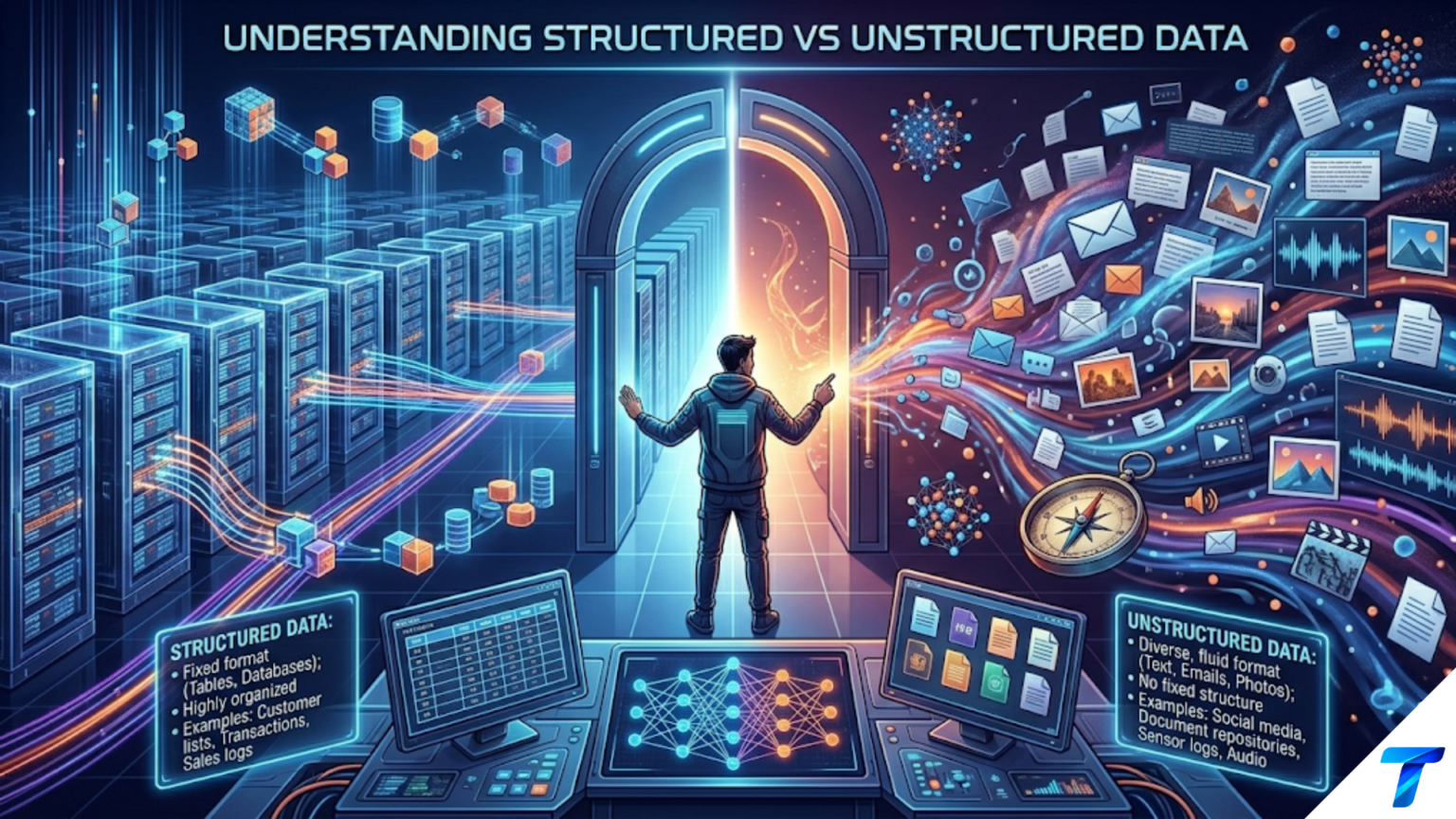
Structured data is information organized into predefined rows and columns with consistent data types — like a spreadsheet or database table — making it directly queryable with SQL and easy to analyze with standard tools. Unstructured data has no predefined format or organization — like text documents, images, audio, and video — and requires specialized preprocessing before analysis. A third category, semi-structured data, falls between the two: it has some organizational markers (like JSON or XML tags) but doesn’t conform to a rigid tabular schema.

Introduction

Walk into any data science team meeting and listen for two minutes. You’ll hear people talking about customer databases, survey responses, product images, support chat logs, social media posts, and sensor readings from IoT devices — all in the same conversation. What most people don’t explicitly say, but implicitly understand, is that these data sources are fundamentally different in their nature. They live in different places, require different tools to process, and pose different analytical challenges.

That fundamental difference is captured by the distinction between structured and unstructured data — one of the most important conceptual frameworks in all of data science. Understanding it isn’t just academic: it directly determines what storage systems you’ll use, what tools and algorithms are appropriate, how you’ll preprocess the data, and what kinds of questions you can ask of it efficiently.

The world generates an astonishing volume of data every day. Industry estimates consistently suggest that 80–90% of all newly generated data is unstructured — text, images, audio, video, sensor streams — while only 10–20% is the neat, tabular, structured data that traditional analytics tools were built to handle. As a data scientist, you’ll need to work fluently across the entire spectrum.

This article gives you a comprehensive understanding of structured, semi-structured, and unstructured data: what each type is, concrete examples from real industries, how they’re stored and processed, their strengths and weaknesses, and how modern data science practice bridges between them.

Structured Data: The Traditional Foundation

What Is Structured Data?

Structured data is information that has been organized into a well-defined format with a fixed schema — a consistent set of fields with specified data types, arranged in rows and columns. Every record follows the same template; every field contains values of the expected type.

Think of a spreadsheet: column headers define what each field represents, and every row is a record with values filling those columns. Scale that concept up to millions of rows with strict enforcement of types and constraints, and you have a relational database — the canonical storage system for structured data.

Characteristics of Structured Data

• Predefined schema: The structure is defined before data is entered — column names, data types, and constraints are set up in advance
• Tabular format: Data is organized in rows (records) and columns (fields/attributes)
• Consistent types: Each column holds values of a specific, consistent data type (integer, float, string, date, boolean)
• Directly queryable: Can be queried with SQL or similar languages without preprocessing
• Quantitative and categorical: Typically contains numbers, dates, and category labels — not free text or media
• Relational: Multiple tables can be linked through shared keys (customer_id, product_id, etc.)

Real-World Examples of Structured Data

Customer transaction records:

Every row is a transaction. Every column has a defined type and meaning. You can query this with SQL in seconds: SELECT customer_id, SUM(amount) FROM transactions GROUP BY customer_id.

Healthcare patient records:

Financial market data:

Other common structured data sources:

• Census data (demographics by geography)
• Weather station readings (temperature, humidity, pressure by time and location)
• Sports statistics (player performance metrics per game)
• E-commerce inventory (product catalog with attributes and prices)
• Web server access logs (though these can also be semi-structured)
• CRM records (contact information, deal stages, revenue figures)

Storage Systems for Structured Data

Structured data is primarily stored in relational database management systems (RDBMS):

• PostgreSQL: Open-source, feature-rich, widely used in data science
• MySQL: Widely deployed for web applications and transactional systems
• SQLite: Lightweight, file-based, excellent for local development and smaller datasets
• SQL Server: Microsoft’s enterprise RDBMS
• Oracle Database: Enterprise systems, especially in finance and healthcare

For analytical workloads on large structured datasets, columnar databases and data warehouses are preferred:

• Amazon Redshift: AWS columnar data warehouse
• Google BigQuery: Serverless, highly scalable analytical database
• Snowflake: Cloud-native data warehouse
• DuckDB: In-process OLAP database, excellent for data science workflows
• Apache Parquet: Columnar file format for analytical storage (not a database, but optimized for analytics)

Analyzing Structured Data

Structured data is the domain where traditional data analysis tools shine. The full toolkit is available:

import pandas as pd
import sqlite3

# Load from CSV (the simplest structured data format)
df = pd.read_csv("transactions.csv")

# Immediate analysis — no preprocessing needed
print(df.groupby('product_category')['amount'].agg(['mean', 'sum', 'count']))

# Load from a relational database
conn = sqlite3.connect("company_data.db")
df = pd.read_sql_query("""
    SELECT 
        customer_id,
        COUNT(*) as num_transactions,
        SUM(amount) as total_spend,
        MAX(date) as last_transaction_date
    FROM transactions
    WHERE date >= '2024-01-01'
    GROUP BY customer_id
    HAVING COUNT(*) >= 3
""", conn)

# Statistical analysis
print(df['total_spend'].describe())
print(df.corr())

import pandas as pd
import sqlite3

# Load from CSV (the simplest structured data format)
df = pd.read_csv("transactions.csv")

# Immediate analysis — no preprocessing needed
print(df.groupby('product_category')['amount'].agg(['mean', 'sum', 'count']))

# Load from a relational database
conn = sqlite3.connect("company_data.db")
df = pd.read_sql_query("""
    SELECT 
        customer_id,
        COUNT(*) as num_transactions,
        SUM(amount) as total_spend,
        MAX(date) as last_transaction_date
    FROM transactions
    WHERE date >= '2024-01-01'
    GROUP BY customer_id
    HAVING COUNT(*) >= 3
""", conn)

# Statistical analysis
print(df['total_spend'].describe())
print(df.corr())

Strengths of structured data:

• Immediately queryable without preprocessing
• Efficient storage and retrieval at scale
• Full range of statistical and ML algorithms applicable
• Easy to understand, validate, and audit
• Excellent tooling (SQL, pandas, Excel)

Limitations of structured data:

• The world doesn’t naturally produce structured data — structuring it takes work
• Rigid schema makes it difficult to capture nuanced, variable information
• Can’t represent rich content (what a product actually looks like, what a customer said)
• Schema changes are costly to implement in production systems

Unstructured Data: The Majority of the World’s Information

What Is Unstructured Data?

Unstructured data is information that doesn’t conform to a predefined data model or organized format. It has no rows and columns, no consistent field names, and often no agreed-upon way to represent its content in a database. The information is embedded within the content itself — a sentence, a pixel, a sound wave, a video frame — rather than in a tabular cell.

This doesn’t mean unstructured data is chaotic or meaningless. A novel is highly organized — it has chapters, paragraphs, sentences, and words — but none of that organization maps to a relational table. An image has precise pixel-level structure — but you can’t put an image in a column and query it with SQL. Unstructured data has structure, just not the kind that tabular databases were designed to exploit.

Types and Examples of Unstructured Data

Text data is the most common form of unstructured data in business:

• Customer reviews and ratings (the text of the review, not the star rating)
• Social media posts and comments
• Email communications
• Customer support chat transcripts
• News articles and blog posts
• Legal contracts and regulatory filings
• Medical notes and clinical reports
• Scientific research papers

Image data:

• Medical imaging (X-rays, MRI scans, CT scans, pathology slides)
• Satellite and aerial photography
• Product photographs in e-commerce catalogs
• Security camera footage (individual frames)
• Social media photos
• Manufacturing quality control images (detecting defects)

Audio data:

• Customer service call recordings
• Podcast content
• Music tracks
• Voice assistant interactions
• Environmental audio (for monitoring industrial equipment)

Video data:

• Surveillance footage
• User-generated content (YouTube, TikTok, Instagram Reels)
• Security recordings
• Training videos and educational content
• Sports broadcast footage

Other unstructured formats:

• PDF documents (often contain structured tables but the overall format is unstructured)
• Presentation files (PowerPoint)
• Geographic data (maps, shapefiles)
• Binary sensor streams

The Challenge: Turning Unstructured Data into Analyzable Information

The fundamental challenge of unstructured data is that most standard analytical tools can’t work with it directly. You can’t run a SQL query on a folder of images. You can’t compute the correlation between two collections of text reviews. You can’t put a video in a DataFrame column and fit a logistic regression to it.

To analyze unstructured data, you must first transform it into structured or numerical representations that algorithms can process. This is the domain of specialized preprocessing techniques:

For text data:

from sklearn.feature_extraction.text import TfidfVectorizer
from transformers import pipeline

reviews = [
    "The product quality is excellent and shipping was fast",
    "Terrible experience, product broke after one day",
    "Decent product but overpriced for what you get"
]

# Method 1: TF-IDF — convert text to numeric feature vectors
vectorizer = TfidfVectorizer(max_features=1000, stop_words='english')
X_tfidf = vectorizer.fit_transform(reviews)
# X_tfidf is now a (3, 1000) matrix — structured, analyzable

# Method 2: Sentiment analysis — extract a structured signal
sentiment_pipeline = pipeline("sentiment-analysis")
sentiments = sentiment_pipeline(reviews)
# [{'label': 'POSITIVE', 'score': 0.9998},
#  {'label': 'NEGATIVE', 'score': 0.9995},
#  {'label': 'NEGATIVE', 'score': 0.8821}]
# Now we have a structured label and confidence score per review

from sklearn.feature_extraction.text import TfidfVectorizer
from transformers import pipeline

reviews = [
    "The product quality is excellent and shipping was fast",
    "Terrible experience, product broke after one day",
    "Decent product but overpriced for what you get"
]

# Method 1: TF-IDF — convert text to numeric feature vectors
vectorizer = TfidfVectorizer(max_features=1000, stop_words='english')
X_tfidf = vectorizer.fit_transform(reviews)
# X_tfidf is now a (3, 1000) matrix — structured, analyzable

# Method 2: Sentiment analysis — extract a structured signal
sentiment_pipeline = pipeline("sentiment-analysis")
sentiments = sentiment_pipeline(reviews)
# [{'label': 'POSITIVE', 'score': 0.9998},
#  {'label': 'NEGATIVE', 'score': 0.9995},
#  {'label': 'NEGATIVE', 'score': 0.8821}]
# Now we have a structured label and confidence score per review

For image data:

from PIL import Image
import numpy as np
from torchvision import transforms, models
import torch

# Method 1: Raw pixels — flatten image to vector
img = Image.open("product_photo.jpg").resize((224, 224))
pixel_array = np.array(img).flatten()  # Shape: (150528,) — structured but very high-dimensional

# Method 2: Deep learning embeddings — extract meaningful features
model = models.resnet50(pretrained=True)
model.eval()

preprocess = transforms.Compose([
    transforms.Resize(256),
    transforms.CenterCrop(224),
    transforms.ToTensor(),
    transforms.Normalize(mean=[0.485, 0.456, 0.406], 
                         std=[0.229, 0.224, 0.225])
])

img_tensor = preprocess(img).unsqueeze(0)
with torch.no_grad():
    embedding = model(img_tensor)
# embedding shape: (1, 1000) — 1000 structured features representing image content

from PIL import Image
import numpy as np
from torchvision import transforms, models
import torch

# Method 1: Raw pixels — flatten image to vector
img = Image.open("product_photo.jpg").resize((224, 224))
pixel_array = np.array(img).flatten()  # Shape: (150528,) — structured but very high-dimensional

# Method 2: Deep learning embeddings — extract meaningful features
model = models.resnet50(pretrained=True)
model.eval()

preprocess = transforms.Compose([
    transforms.Resize(256),
    transforms.CenterCrop(224),
    transforms.ToTensor(),
    transforms.Normalize(mean=[0.485, 0.456, 0.406], 
                         std=[0.229, 0.224, 0.225])
])

img_tensor = preprocess(img).unsqueeze(0)
with torch.no_grad():
    embedding = model(img_tensor)
# embedding shape: (1, 1000) — 1000 structured features representing image content

For audio data:

import librosa
import numpy as np

# Load audio file
audio, sample_rate = librosa.load("call_recording.wav")

# Extract structured features (MFCCs — Mel-Frequency Cepstral Coefficients)
mfccs = librosa.feature.mfcc(y=audio, sr=sample_rate, n_mfcc=40)
# mfccs shape: (40, time_steps) — structured feature matrix

# Summary statistics create a fixed-length feature vector
mfcc_features = np.concatenate([
    mfccs.mean(axis=1),    # Mean of each coefficient across time
    mfccs.std(axis=1),     # Std of each coefficient
    mfccs.max(axis=1)      # Max of each coefficient
])
# mfcc_features shape: (120,) — fixed-length structured vector

import librosa
import numpy as np

# Load audio file
audio, sample_rate = librosa.load("call_recording.wav")

# Extract structured features (MFCCs — Mel-Frequency Cepstral Coefficients)
mfccs = librosa.feature.mfcc(y=audio, sr=sample_rate, n_mfcc=40)
# mfccs shape: (40, time_steps) — structured feature matrix

# Summary statistics create a fixed-length feature vector
mfcc_features = np.concatenate([
    mfccs.mean(axis=1),    # Mean of each coefficient across time
    mfccs.std(axis=1),     # Std of each coefficient
    mfccs.max(axis=1)      # Max of each coefficient
])
# mfcc_features shape: (120,) — fixed-length structured vector

The pattern is consistent: unstructured → feature extraction → structured numerical representation → standard ML algorithms.

Storage Systems for Unstructured Data

Because unstructured data can’t be stored in tabular databases, different storage systems are used:

Object/blob storage (most common for large-scale unstructured data):

• Amazon S3: The dominant cloud object store — images, videos, documents stored as binary objects
• Google Cloud Storage: Google’s equivalent
• Azure Blob Storage: Microsoft’s equivalent
• MinIO: Self-hosted, S3-compatible open-source alternative

Document databases (for text and semi-structured data):

• MongoDB: Stores JSON-like documents — excellent for text and hierarchical data
• Elasticsearch: Specialized for full-text search across large document collections
• Apache Solr: Another full-text search engine

Specialized databases:

• Pinecone, Weaviate, Chroma: Vector databases for storing and querying embeddings (the numerical representations of unstructured data)
• Cassandra: Wide-column store for high-write workloads
• Neo4j: Graph database for relationship-heavy data (social networks, knowledge graphs)

Semi-Structured Data: The Middle Ground

What Is Semi-Structured Data?

Semi-structured data occupies the space between structured and unstructured. It has self-describing structure — organizational markers that identify fields and their relationships — but it doesn’t conform to the rigid, predefined schema of a relational table. The schema is flexible: records can have different fields, fields can be nested hierarchically, and arrays can hold variable numbers of elements.

The defining characteristic: the data carries its own structural metadata. You don’t need a separate schema document to understand the organization — the tags, keys, and markers are embedded in the data itself.

JSON: The Most Common Semi-Structured Format

JSON (JavaScript Object Notation) is the dominant format for semi-structured data in modern applications — especially web APIs, event streams, and NoSQL databases.

{
  "customer_id": "CUST_8821",
  "name": "Jane Smith",
  "email": "jane.smith@example.com",
  "address": {
    "street": "123 Oak Avenue",
    "city": "Austin",
    "state": "TX",
    "zip": "78701"
  },
  "preferences": {
    "notification_channel": "email",
    "categories_of_interest": ["electronics", "home", "books"]
  },
  "transactions": [
    {
      "id": "TXN_001",
      "date": "2024-09-01",
      "amount": 149.99,
      "items": [
        {"product_id": "PROD_001", "quantity": 1, "price": 149.99}
      ]
    },
    {
      "id": "TXN_002",
      "date": "2024-09-15",
      "amount": 534.00,
      "items": [
        {"product_id": "PROD_047", "quantity": 2, "price": 199.00},
        {"product_id": "PROD_112", "quantity": 1, "price": 136.00}
      ]
    }
  ],
  "account_created": "2022-03-14",
  "is_premium": true,
  "lifetime_value": 3847.50
}

{
  "customer_id": "CUST_8821",
  "name": "Jane Smith",
  "email": "jane.smith@example.com",
  "address": {
    "street": "123 Oak Avenue",
    "city": "Austin",
    "state": "TX",
    "zip": "78701"
  },
  "preferences": {
    "notification_channel": "email",
    "categories_of_interest": ["electronics", "home", "books"]
  },
  "transactions": [
    {
      "id": "TXN_001",
      "date": "2024-09-01",
      "amount": 149.99,
      "items": [
        {"product_id": "PROD_001", "quantity": 1, "price": 149.99}
      ]
    },
    {
      "id": "TXN_002",
      "date": "2024-09-15",
      "amount": 534.00,
      "items": [
        {"product_id": "PROD_047", "quantity": 2, "price": 199.00},
        {"product_id": "PROD_112", "quantity": 1, "price": 136.00}
      ]
    }
  ],
  "account_created": "2022-03-14",
  "is_premium": true,
  "lifetime_value": 3847.50
}

This is clearly organized — but it can’t be directly put in a relational table because:

• The address field is itself a nested object
• categories_of_interest is an array of variable length
• transactions contains a nested array of transaction objects, each with its own nested items array
• Different customers might have different subsets of these fields

XML: The Older Semi-Structured Standard

XML (eXtensible Markup Language) was the dominant semi-structured format before JSON, and remains widely used in enterprise systems, healthcare (HL7/FHIR), financial data (FIX protocol), and document formats (Microsoft Office files are ZIP archives of XML):

<patient id="P_0001">
  <demographics>
    <age>54</age>
    <gender>Male</gender>
    <blood_type>A+</blood_type>
  </demographics>
  <diagnoses>
    <diagnosis code="I10" description="Essential hypertension" date="2024-08-15"/>
    <diagnosis code="E11.9" description="Type 2 diabetes" date="2023-11-02"/>
  </diagnoses>
  <medications>
    <medication name="Lisinopril" dose="10mg" frequency="daily" since="2024-08-20"/>
  </medications>
  <notes>
    Patient reports improved blood pressure control since starting Lisinopril.
    Follow up in 3 months.
  </notes>
</patient>

<patient id="P_0001">
  <demographics>
    <age>54</age>
    <gender>Male</gender>
    <blood_type>A+</blood_type>
  </demographics>
  <diagnoses>
    <diagnosis code="I10" description="Essential hypertension" date="2024-08-15"/>
    <diagnosis code="E11.9" description="Type 2 diabetes" date="2023-11-02"/>
  </diagnoses>
  <medications>
    <medication name="Lisinopril" dose="10mg" frequency="daily" since="2024-08-20"/>
  </medications>
  <notes>
    Patient reports improved blood pressure control since starting Lisinopril.
    Follow up in 3 months.
  </notes>
</patient>

Other Semi-Structured Formats

YAML is used extensively for configuration files and data science experiment configs:

experiment:
  name: customer_churn_v3
  model:
    type: xgboost
    params:
      n_estimators: 500
      learning_rate: 0.05

experiment:
  name: customer_churn_v3
  model:
    type: xgboost
    params:
      n_estimators: 500
      learning_rate: 0.05

CSV with nested values is technically structured but becomes semi-structured when cells contain JSON strings, arrays, or other complex objects:

customer_id,name,tags,metadata
CUST_001,Jane,["loyal","premium"],{"tier": 3, "since": 2020}

customer_id,name,tags,metadata
CUST_001,Jane,["loyal","premium"],{"tier": 3, "since": 2020}

Parquet files can store complex nested structures (arrays, maps, structs) beyond what flat CSV can represent.

Log files are often semi-structured — they have consistent patterns (timestamps, log levels) but variable message content:

2024-09-15 14:23:11 INFO  [api_gateway] Request received: POST /api/predict
2024-09-15 14:23:11 DEBUG [preprocessing] Input shape: (1, 47)
2024-09-15 14:23:12 INFO  [model_server] Prediction: 0.742 (latency: 87ms)
2024-09-15 14:23:15 ERROR [api_gateway] Timeout after 4000ms for request_id=abc123

2024-09-15 14:23:11 INFO  [api_gateway] Request received: POST /api/predict
2024-09-15 14:23:11 DEBUG [preprocessing] Input shape: (1, 47)
2024-09-15 14:23:12 INFO  [model_server] Prediction: 0.742 (latency: 87ms)
2024-09-15 14:23:15 ERROR [api_gateway] Timeout after 4000ms for request_id=abc123

Working with Semi-Structured Data in Python

import json
import pandas as pd
from pathlib import Path

# Load JSON
with open("customers.json", 'r') as f:
    customer = json.load(f)

# Access nested fields
city = customer['address']['city']          # "Austin"
categories = customer['preferences']['categories_of_interest']  # ['electronics', 'home', 'books']
first_txn_amount = customer['transactions'][0]['amount']         # 149.99

# Flatten nested JSON to a DataFrame — pandas json_normalize
from pandas import json_normalize

# Flatten address into separate columns
df = json_normalize(customer)
# Produces columns: customer_id, name, address.city, address.state, etc.

# Flatten transactions array — one row per transaction
df_transactions = json_normalize(
    customer,
    record_path='transactions',
    meta=['customer_id', 'name']
)

# Working with JSON in pandas directly
# Reading a JSON Lines file (each line is a separate JSON object)
df = pd.read_json("events.jsonl", lines=True)

# Exploding nested list columns
df_exploded = df.explode('categories_of_interest')

# Accessing dict columns
df['city'] = df['address'].apply(lambda x: x.get('city') if isinstance(x, dict) else None)

import json
import pandas as pd
from pathlib import Path

# Load JSON
with open("customers.json", 'r') as f:
    customer = json.load(f)

# Access nested fields
city = customer['address']['city']          # "Austin"
categories = customer['preferences']['categories_of_interest']  # ['electronics', 'home', 'books']
first_txn_amount = customer['transactions'][0]['amount']         # 149.99

# Flatten nested JSON to a DataFrame — pandas json_normalize
from pandas import json_normalize

# Flatten address into separate columns
df = json_normalize(customer)
# Produces columns: customer_id, name, address.city, address.state, etc.

# Flatten transactions array — one row per transaction
df_transactions = json_normalize(
    customer,
    record_path='transactions',
    meta=['customer_id', 'name']
)

# Working with JSON in pandas directly
# Reading a JSON Lines file (each line is a separate JSON object)
df = pd.read_json("events.jsonl", lines=True)

# Exploding nested list columns
df_exploded = df.explode('categories_of_interest')

# Accessing dict columns
df['city'] = df['address'].apply(lambda x: x.get('city') if isinstance(x, dict) else None)

import xml.etree.ElementTree as ET

# Parse XML
tree = ET.parse("patients.xml")
root = tree.getroot()

# Extract data into structured format
records = []
for patient in root.findall('patient'):
    record = {
        'patient_id': patient.get('id'),
        'age': patient.find('demographics/age').text,
        'gender': patient.find('demographics/gender').text
    }
    
    # Extract multiple diagnoses
    diagnoses = [
        diag.get('code')
        for diag in patient.findall('diagnoses/diagnosis')
    ]
    record['diagnosis_codes'] = diagnoses
    record['n_diagnoses'] = len(diagnoses)
    
    records.append(record)

df_patients = pd.DataFrame(records)

import xml.etree.ElementTree as ET

# Parse XML
tree = ET.parse("patients.xml")
root = tree.getroot()

# Extract data into structured format
records = []
for patient in root.findall('patient'):
    record = {
        'patient_id': patient.get('id'),
        'age': patient.find('demographics/age').text,
        'gender': patient.find('demographics/gender').text
    }
    
    # Extract multiple diagnoses
    diagnoses = [
        diag.get('code')
        for diag in patient.findall('diagnoses/diagnosis')
    ]
    record['diagnosis_codes'] = diagnoses
    record['n_diagnoses'] = len(diagnoses)
    
    records.append(record)

df_patients = pd.DataFrame(records)

The Three Types: A Comprehensive Comparison

Industry Applications: Where Each Data Type Dominates

Finance

Structured: Stock prices, trade records, account balances, transaction histories, credit scores — the backbone of traditional financial analytics.

Semi-structured: Trading API responses (JSON), regulatory filings in XBRL format, market data feeds.

Unstructured: Earnings call transcripts (NLP for sentiment and guidance extraction), analyst research reports, news articles that move markets, SEC filing text bodies.

A hedge fund might combine all three: structured price data, semi-structured news event data from JSON APIs, and unstructured news article sentiment to build a trading signal.

Healthcare

Structured: Lab results, vital signs, procedure codes (ICD-10), billing data, medication dosage records — the RDBMS core of hospital information systems.

Semi-structured: HL7 FHIR patient records, medical device data streams, prescription refill histories in XML.

Unstructured: Clinical notes (the rich, narrative descriptions doctors write), medical imaging (X-rays, MRIs), pathology slide images, patient-reported outcomes in free text.

A clinical AI system might use structured lab values to flag abnormal results, semi-structured FHIR records to understand medication history, and NLP on clinical notes to extract symptoms not captured in structured codes.

E-commerce and Retail

Structured: Sales transactions, inventory levels, pricing history, customer account data, shipment tracking numbers.

Semi-structured: Product catalog data (nested attributes vary by category — a laptop has CPU, RAM, storage specs; a shirt has size, color, material), clickstream events (JSON), A/B test results.

Unstructured: Product images (visual search, quality inspection), customer reviews (sentiment, topic extraction), social media mentions, product description text.

Amazon’s recommendation engine combines purchase history (structured), browsing behavior (semi-structured event logs), and product images plus description text (unstructured) to generate personalized recommendations.

Manufacturing and Industry

Structured: Production quantities, defect rates, maintenance schedules, supplier data, cost tracking.

Semi-structured: IoT sensor data streams (JSON events from equipment), quality control inspection records.

Unstructured: Quality inspection images (computer vision for defect detection), equipment sound signatures (audio ML for predictive maintenance), engineering documents and manuals (NLP for maintenance guidance).

A factory floor predictive maintenance system might combine structured maintenance records with unstructured vibration sensor audio and inspection camera images to predict equipment failures before they occur.

The Convergence: Modern Data Science Bridges All Three

In contemporary data science practice, the boundary between structured and unstructured data has become increasingly porous, for two reasons.

Reason 1: Feature Extraction Creates Structure from Unstructured Data

The dominant paradigm in modern ML — transfer learning and embedding-based methods — transforms unstructured data into rich numerical representations (embeddings) that can be stored in regular databases and analyzed with standard ML tools.

from sentence_transformers import SentenceTransformer

# Unstructured text → dense numerical embeddings
model = SentenceTransformer('all-MiniLM-L6-v2')

customer_reviews = [
    "The product quality is excellent but shipping took too long",
    "Worst purchase I've ever made — completely broken on arrival",
    "Pretty good value for money, would buy again"
]

# Each review becomes a 384-dimensional vector
embeddings = model.encode(customer_reviews)
# embeddings shape: (3, 384) — now structured!

# These embeddings can be stored in a vector database
# and queried by semantic similarity
import chromadb

client = chromadb.Client()
collection = client.create_collection("reviews")

collection.add(
    documents=customer_reviews,
    embeddings=embeddings.tolist(),
    ids=["review_1", "review_2", "review_3"]
)

# Query: find reviews semantically similar to "delivery problems"
results = collection.query(
    query_texts=["slow delivery and shipping issues"],
    n_results=2
)

from sentence_transformers import SentenceTransformer

# Unstructured text → dense numerical embeddings
model = SentenceTransformer('all-MiniLM-L6-v2')

customer_reviews = [
    "The product quality is excellent but shipping took too long",
    "Worst purchase I've ever made — completely broken on arrival",
    "Pretty good value for money, would buy again"
]

# Each review becomes a 384-dimensional vector
embeddings = model.encode(customer_reviews)
# embeddings shape: (3, 384) — now structured!

# These embeddings can be stored in a vector database
# and queried by semantic similarity
import chromadb

client = chromadb.Client()
collection = client.create_collection("reviews")

collection.add(
    documents=customer_reviews,
    embeddings=embeddings.tolist(),
    ids=["review_1", "review_2", "review_3"]
)

# Query: find reviews semantically similar to "delivery problems"
results = collection.query(
    query_texts=["slow delivery and shipping issues"],
    n_results=2
)

Reason 2: Multi-Modal Models Process All Data Types Together

State-of-the-art models like GPT-4V, DALL-E, and Gemini accept multiple input modalities — text, images, and structured data — in a single prompt, further blurring the distinction from a model’s perspective (though the underlying storage and preprocessing requirements remain distinct).

The Modern Data Stack Handles All Three

Modern data infrastructure — the “data lakehouse” architecture — is designed to store and query all three data types from a unified platform:

Raw Data Layer (Data Lake — usually S3):
├── structured/          ← CSV, Parquet files
├── semi-structured/     ← JSON, XML, log files
└── unstructured/        ← images/, audio/, documents/

Processing Layer:
├── Spark / Databricks   ← Process all three types at scale
├── dbt                  ← Transform structured data
└── Feature pipelines    ← Extract features from unstructured

Analytics Layer:
├── Snowflake / BigQuery ← Analyze structured + semi-structured
├── Vector DB (Pinecone) ← Search unstructured via embeddings
└── BI Tools (Tableau)   ← Visualize structured outputs

Raw Data Layer (Data Lake — usually S3):
├── structured/          ← CSV, Parquet files
├── semi-structured/     ← JSON, XML, log files
└── unstructured/        ← images/, audio/, documents/

Processing Layer:
├── Spark / Databricks   ← Process all three types at scale
├── dbt                  ← Transform structured data
└── Feature pipelines    ← Extract features from unstructured

Analytics Layer:
├── Snowflake / BigQuery ← Analyze structured + semi-structured
├── Vector DB (Pinecone) ← Search unstructured via embeddings
└── BI Tools (Tableau)   ← Visualize structured outputs

Practical Guidance: Working with Each Type in Data Science

Identifying Your Data Type at the Start of a Project

Before diving into analysis, always identify what type of data you’re working with — it determines your entire approach:

Ask these questions:

1. Does every record have the same fields? → If yes, likely structured
2. Can it be directly loaded into a pandas DataFrame without preprocessing? → If yes, likely structured or semi-structured
3. Are there nested objects or arrays within records? → Semi-structured
4. Is it images, audio, video, or free text? → Unstructured
5. Does it require specialized models (NLP, computer vision) to extract meaning? → Unstructured

Knowing When to Combine Data Types

The most sophisticated and powerful data science work often combines all three types. Building a customer churn model with high accuracy might require:

• Structured data: Transaction history (RFM metrics), account age, plan type
• Semi-structured data: App usage event logs (frequency and type of interactions), support ticket metadata
• Unstructured data: Sentiment from support chat transcripts, theme analysis from cancellation survey responses

Each type contributes signal that the others can’t provide. The structured data gives precise behavioral metrics; the semi-structured event logs reveal usage patterns; the unstructured text reveals why customers are dissatisfied — the voice of the customer that no structured field captures.

Summary

The distinction between structured, semi-structured, and unstructured data is foundational to data science because it determines how data must be stored, queried, preprocessed, and modeled. Structured data — organized in rows and columns with a rigid schema — is the natural domain of SQL, relational databases, and traditional statistical methods. Unstructured data — images, audio, video, free text — requires feature extraction through computer vision, NLP, or signal processing before standard algorithms can be applied. Semi-structured data occupies the middle ground, with self-describing organization like JSON or XML that is flexible but requires parsing and potentially flattening before tabular analysis.

In practice, the world’s most valuable analytical insights often come from combining all three: structured behavioral data provides the quantitative foundation, semi-structured event and API data captures the interactions, and unstructured text and media reveals the qualitative context that numbers alone can’t convey. Modern data science tools and infrastructure increasingly support working fluently across the entire spectrum — from SQL databases for structured data to vector databases for unstructured embeddings — making the ability to work with all three types a core professional competency.

Key Takeaways

• Structured data follows a predefined schema with consistent rows and columns, is directly queryable with SQL, and requires minimal preprocessing — examples include transaction records, sensor readings, and financial market data
• Unstructured data has no predefined format and cannot be directly analyzed by most ML algorithms — it must first be transformed into numerical representations through feature extraction methods specific to each data type (TF-IDF or embeddings for text, pixel arrays or CNN features for images, MFCCs for audio)
• Semi-structured data carries its own organizational markers (JSON keys, XML tags) making it self-describing and flexible, but typically requires parsing and flattening before tabular analysis
• An estimated 80–90% of newly generated data worldwide is unstructured — images, video, audio, and text — making the ability to work with unstructured data a critical modern data science skill
• The choice of storage system depends on data type: relational databases and data warehouses for structured, object stores and document databases for unstructured and semi-structured, and vector databases for storing and querying embeddings derived from unstructured data
• The most powerful real-world data science applications combine all three data types: structured metrics provide the quantitative foundation, semi-structured event data captures interactions, and unstructured text and media reveals qualitative context
• Modern transfer learning and embedding models have largely dissolved the analytical boundary between structured and unstructured data — converting images, text, and audio into rich numerical vectors that can be stored in databases and analyzed with standard ML tools