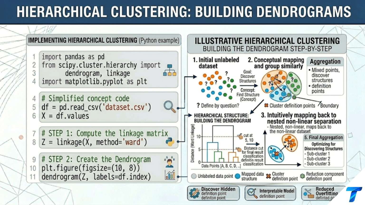
Hierarchical clustering builds a tree (dendrogram) of nested cluster relationships without requiring you to specify the number of clusters in advance. Agglomerative (bottom-up) clustering starts with each point as its own cluster and merges the two closest clusters at each step. Divisive (top-down) clustering starts with all points in one cluster and recursively splits. You choose the final number of clusters by cutting the dendrogram horizontally at any level — different heights reveal different granularities of the same hierarchical structure.
Introduction
K-Means forces a fundamental decision before clustering begins: specify k. This is inconvenient when you don’t know how many clusters exist, and limiting when clusters exist at multiple scales simultaneously — a dataset of news articles might cluster into 5 broad topics or 50 specific subtopics, and both views are valid.
Hierarchical clustering offers a fundamentally different philosophy: rather than partitioning data into exactly k clusters, it builds a complete tree of merges (or splits) from which any level of granularity can be read. A biologist grouping animal species can read the dendrogram at the level of genus, family, order, or class — each cut of the tree reveals a different but equally valid taxonomy. A marketing analyst can cut the customer dendrogram at 5 clusters for a broad strategy or 20 clusters for a precision campaign.
The result is a dendrogram — a visual tree diagram where the height of each merge reflects the dissimilarity between the groups being merged. Similar points merge early (low on the tree) at small heights. Dissimilar groups merge late (high on the tree) at large heights. The structure of the dendrogram itself is informative — long branches indicate well-separated groups; short branches indicate that nearby points merged at similar distances.
This article covers the complete theory and implementation of hierarchical clustering: the agglomerative algorithm, every major linkage criterion and when each fails, dendrogram interpretation, cutting strategies, practical Python implementation with scipy and scikit-learn, and a comparison with K-Means.
The Agglomerative Algorithm
Agglomerative hierarchical clustering builds the dendrogram bottom-up:
- Start: each of the n data points is its own cluster (n clusters total)
- Compute all pairwise distances between clusters
- Merge the two closest clusters into one
- Update the distance matrix (using the chosen linkage criterion)
- Repeat steps 3–4 until only one cluster remains
The result is a complete binary tree of n−1 merges.
import numpy as np
import matplotlib.pyplot as plt
from scipy.cluster.hierarchy import dendrogram, linkage, fcluster
from scipy.spatial.distance import pdist, squareform
from sklearn.preprocessing import StandardScaler
from sklearn.datasets import make_blobs
import warnings
warnings.filterwarnings('ignore')

np.random.seed(42)


class AgglomerativeFromScratch:
    """
    Agglomerative hierarchical clustering implemented from scratch.
    Tracks every merge step for educational visualization.
    Supports single, complete, average, and Ward linkage.
    """

    def __init__(self, linkage='ward'):
        """
        Args:
            linkage: 'single', 'complete', 'average', or 'ward'
        """
        self.linkage_  = linkage
        self.merges_   = []   # List of (cluster_a, cluster_b, distance, size)
        self.labels_   = None

    def _cluster_distance(self, C_a, C_b, X, dist_matrix):
        """
        Compute distance between two clusters using the specified linkage.

        Single:   min distance between any pair of points across clusters
        Complete: max distance between any pair of points across clusters
        Average:  mean distance between all pairs (UPGMA)
        Ward:     increase in total WCSS from merging (variance-based)
        """
        a_pts = list(C_a)
        b_pts = list(C_b)

        if self.linkage_ == 'single':
            return min(dist_matrix[i, j] for i in a_pts for j in b_pts)

        elif self.linkage_ == 'complete':
            return max(dist_matrix[i, j] for i in a_pts for j in b_pts)

        elif self.linkage_ == 'average':
            total = sum(dist_matrix[i, j] for i in a_pts for j in b_pts)
            return total / (len(a_pts) * len(b_pts))

        elif self.linkage_ == 'ward':
            # Ward linkage: increase in WCSS from merging A and B
            n_a = len(a_pts)
            n_b = len(b_pts)
            mu_a = X[a_pts].mean(axis=0)
            mu_b = X[b_pts].mean(axis=0)
            # Ward distance formula
            return np.sqrt(n_a * n_b / (n_a + n_b)) * np.linalg.norm(mu_a - mu_b)

        else:
            raise ValueError(f"Unknown linkage: {self.linkage_}")

    def fit(self, X):
        """Build the dendrogram by repeatedly merging nearest clusters."""
        n = len(X)
        # Precompute pairwise distances
        dist_matrix = squareform(pdist(X, metric='euclidean'))

        # Each point starts as its own cluster (stored as a frozenset of indices)
        clusters    = {i: frozenset([i]) for i in range(n)}
        cluster_ids = list(range(n))
        self.merges_ = []

        while len(clusters) > 1:
            # Find the two closest clusters
            min_dist = np.inf
            merge_a  = None
            merge_b  = None

            ids = list(clusters.keys())
            for i in range(len(ids)):
                for j in range(i + 1, len(ids)):
                    a, b = ids[i], ids[j]
                    d    = self._cluster_distance(
                        clusters[a], clusters[b], X, dist_matrix
                    )
                    if d < min_dist:
                        min_dist = d
                        merge_a  = a
                        merge_b  = b

            # Merge
            new_cluster = clusters[merge_a] | clusters[merge_b]
            new_id      = max(clusters.keys()) + 1
            size        = len(new_cluster)

            self.merges_.append((merge_a, merge_b, min_dist, size))

            # Update clusters
            del clusters[merge_a]
            del clusters[merge_b]
            clusters[new_id] = new_cluster

        return self


# Validate against scipy on a small dataset
print("=== Agglomerative From Scratch: Validation ===\n")

np.random.seed(42)
X_small = np.array([
    [1.0, 1.0], [1.5, 1.2], [2.0, 1.0],   # Cluster A
    [6.0, 5.0], [6.5, 5.5], [7.0, 5.0],   # Cluster B
    [3.5, 8.0], [4.0, 7.5],               # Cluster C
])
X_small_s = StandardScaler().fit_transform(X_small)

for link in ['single', 'complete', 'average', 'ward']:
    hc = AgglomerativeFromScratch(linkage=link)
    hc.fit(X_small_s)

    print(f"  Linkage: {link}")
    print(f"  {'Step':>5} | {'Merge A':>8} | {'Merge B':>8} | {'Distance':>10} | "
          f"{'New Size':>9}")
    print(f"  {'-'*48}")
    for step, (a, b, dist, size) in enumerate(hc.merges_, 1):
        print(f"  {step:>5} | {a:>8} | {b:>8} | {dist:>10.4f} | {size:>9}")
print()Linkage Criteria: The Critical Choice
The linkage criterion defines how the distance between two clusters is measured. This is the most important hyperparameter in hierarchical clustering — different linkages produce qualitatively different dendrograms and cluster shapes.
import numpy as np
import matplotlib.pyplot as plt
from scipy.cluster.hierarchy import dendrogram, linkage, fcluster
from sklearn.preprocessing import StandardScaler
from sklearn.datasets import make_blobs, make_moons


def compare_linkage_criteria(X_s, y_true, title="Dataset", figsize=(20, 12)):
    """
    Side-by-side comparison of four linkage criteria on the same dataset.
    Shows both the dendrogram structure and the resulting cluster assignments
    when the tree is cut to the true number of clusters.
    """
    linkage_methods = ['single', 'complete', 'average', 'ward']
    linkage_labels  = [
        'Single Linkage\n(Min distance — "chaining")',
        'Complete Linkage\n(Max distance — "compactness")',
        'Average Linkage\n(Mean distance — UPGMA)',
        'Ward Linkage\n(Min variance increase)',
    ]

    k_true = len(np.unique(y_true))
    fig, axes = plt.subplots(2, 4, figsize=figsize)

    cluster_colors = ['#e74c3c', '#3498db', '#2ecc71', '#f39c12', '#9b59b6']

    for col, (method, label) in enumerate(zip(linkage_methods, linkage_labels)):
        # Row 0: Dendrogram
        ax_dend = axes[0, col]
        Z = linkage(X_s, method=method)
        dendrogram(
            Z, ax=ax_dend,
            truncate_mode='lastp', p=20,
            show_leaf_counts=True,
            leaf_rotation=90,
            leaf_font_size=7,
            color_threshold=Z[-k_true, 2],  # Color at the k_true-cluster cut
        )
        ax_dend.axhline(y=Z[-k_true, 2], color='coral', linestyle='--',
                         lw=1.5, alpha=0.8, label=f'Cut at k={k_true}')
        ax_dend.set_title(label, fontsize=9, fontweight='bold')
        ax_dend.set_ylabel('Distance' if col == 0 else '', fontsize=9)
        ax_dend.tick_params(axis='x', labelsize=7)
        ax_dend.legend(fontsize=7)

        # Row 1: Scatter plot of cluster assignments
        ax_scat = axes[1, col]
        labels  = fcluster(Z, t=k_true, criterion='maxclust') - 1  # 0-indexed

        from sklearn.metrics import adjusted_rand_score
        ari = adjusted_rand_score(y_true, labels)

        for cls in range(k_true):
            mask = labels == cls
            ax_scat.scatter(X_s[mask, 0], X_s[mask, 1],
                            c=cluster_colors[cls % len(cluster_colors)],
                            s=40, edgecolors='white', linewidth=0.4,
                            alpha=0.85)
        ax_scat.set_title(f'Clusters (ARI={ari:.3f})',
                           fontsize=9, fontweight='bold')
        if col == 0:
            ax_scat.set_xlabel('Feature 1', fontsize=8)
            ax_scat.set_ylabel('Feature 2', fontsize=8)
        ax_scat.grid(True, alpha=0.2)

    plt.suptitle(f'Four Linkage Criteria: {title}\n'
                 'Row 1: Dendrograms | Row 2: Cluster Assignments at k={}'.format(k_true),
                 fontsize=13, fontweight='bold', y=1.01)
    plt.tight_layout()
    plt.savefig(f'linkage_comparison_{title.lower().replace(" ", "_")}.png',
                dpi=150, bbox_inches='tight')
    plt.show()
    print(f"Saved linkage comparison plot.")


# Test on blobs (spherical clusters)
np.random.seed(42)
X_blobs, y_blobs = make_blobs(n_samples=150, centers=3, cluster_std=0.7,
                               random_state=42)
X_blobs_s = StandardScaler().fit_transform(X_blobs)
compare_linkage_criteria(X_blobs_s, y_blobs, title="Spherical Blobs (k=3)")

# Test on moons (non-spherical)
X_moons, y_moons = make_moons(n_samples=150, noise=0.1, random_state=42)
X_moons_s = StandardScaler().fit_transform(X_moons)
compare_linkage_criteria(X_moons_s, y_moons, title="Two Moons")Linkage Criterion Properties
| Linkage | Distance definition | Cluster shape | Sensitivity | Best for |
|---|---|---|---|---|
| Single | min(d(a,b)) for a∈A, b∈B | Elongated chains | Outliers (chaining effect) | Manifold/filament data |
| Complete | max(d(a,b)) for a∈A, b∈B | Compact, equal-size | Outliers (forced into clusters) | Compact, spherical clusters |
| Average | mean(d(a,b)) for a∈A, b∈B | Balanced | Moderate | General purpose |
| Ward | min increase in WCSS | Compact, spherical | Outliers break compactness | Compact clusters, default choice |
Ward linkage is the default choice for most applications because it minimizes the total within-cluster variance at each merge — conceptually equivalent to K-Means’ objective but solved hierarchically. Single linkage should be used when clusters have elongated or manifold shapes but avoided otherwise due to the chaining effect.
Reading Dendrograms
A dendrogram encodes the complete clustering hierarchy. Understanding how to read it is essential for interpreting hierarchical clustering results.
import numpy as np
import matplotlib.pyplot as plt
from scipy.cluster.hierarchy import dendrogram, linkage, fcluster, cophenet
from scipy.spatial.distance import pdist
from sklearn.preprocessing import StandardScaler
from sklearn.datasets import load_iris


def annotated_dendrogram(X_s, labels_true=None, names=None,
                           method='ward', title="Annotated Dendrogram",
                           figsize=(16, 8)):
    """
    Create a fully annotated dendrogram with educational callouts.

    Reading guide:
    - Height of merge: dissimilarity between the merging clusters
    - Long vertical line: the two groups are very different — good separator
    - Short vertical line: groups were similar — uncertain separation
    - Colored regions: distinct subtrees when cut at a given height
    - Leaves: individual data points (or small groups if truncated)
    """
    Z = linkage(X_s, method=method)

    # Cophenetic correlation: how well does the dendrogram preserve distances?
    c, coph_dists = cophenet(Z, pdist(X_s))

    fig, (ax1, ax2) = plt.subplots(1, 2, figsize=figsize,
                                    gridspec_kw={'width_ratios': [2, 1]})

    # ── Left: Full annotated dendrogram ──────────────────────────
    # Suggest a cut level: where is there the longest gap between merges?
    heights = Z[:, 2]
    height_diffs = np.diff(heights)
    cut_idx  = np.argmax(height_diffs[-5:]) - 5  # Among the top merges
    cut_height = (heights[-2] + heights[-1]) / 2  # Default: 2 clusters

    # Find "best" cut: largest gap in top 8 merges
    top_8 = heights[-8:]
    gaps  = np.diff(top_8)
    best_gap_idx = np.argmax(gaps) + len(heights) - 8
    best_cut_height = (heights[best_gap_idx] + heights[best_gap_idx + 1]) / 2

    k_at_best_cut = len(np.unique(fcluster(Z, t=best_cut_height,
                                            criterion='distance')))

    dend_result = dendrogram(
        Z, ax=ax1,
        orientation='top',
        truncate_mode='lastp', p=30,
        show_leaf_counts=True,
        leaf_rotation=90,
        leaf_font_size=8,
        color_threshold=best_cut_height,
        above_threshold_color='gray',
        labels=names,
    )

    # Annotate the cut line
    ax1.axhline(y=best_cut_height, color='coral', linestyle='--', lw=2.5,
                label=f'Suggested cut → k={k_at_best_cut} clusters')
    ax1.set_title(f'{title}\n'
                  f'Cophenetic r = {c:.4f} | Method: {method} | '
                  f'Suggested k = {k_at_best_cut}',
                  fontsize=10, fontweight='bold')
    ax1.set_ylabel('Distance (merge height)', fontsize=11)
    ax1.legend(fontsize=9)

    # Annotate largest gap
    top_k = min(20, len(heights))
    ax1.annotate(
        f'Largest gap\n(cut here\nfor k={k_at_best_cut})',
        xy=(ax1.get_xlim()[1] * 0.6, best_cut_height),
        xytext=(ax1.get_xlim()[1] * 0.75, best_cut_height * 1.3),
        fontsize=8, color='coral',
        arrowprops=dict(arrowstyle='->', color='coral', lw=1.5)
    )

    # ── Right: Height histogram — where are the merges? ──────────
    ax2.barh(range(len(heights[-15:])), heights[-15:],
             color='steelblue', edgecolor='white', linewidth=0.5)
    ax2.axvline(x=best_cut_height, color='coral', linestyle='--', lw=2,
                label='Suggested cut')
    ax2.set_xlabel('Merge height (distance)', fontsize=10)
    ax2.set_ylabel('Merge step (recent)', fontsize=10)
    ax2.set_title('Last 15 Merge Heights\n(Large gap = natural separation)',
                  fontsize=9, fontweight='bold')
    ax2.legend(fontsize=8)
    ax2.invert_yaxis()

    plt.suptitle(f'Dendrogram Reading Guide: {title}',
                 fontsize=13, fontweight='bold')
    plt.tight_layout()
    plt.savefig('dendrogram_annotated.png', dpi=150, bbox_inches='tight')
    plt.show()
    print("Saved: dendrogram_annotated.png")

    print(f"\n  Cophenetic correlation: {c:.4f}")
    print(f"  (Range [0,1] — closer to 1 = dendrogram preserves true distances)")
    if c > 0.8:
        print(f"  → Strong: dendrogram is a faithful representation of the data")
    elif c > 0.6:
        print(f"  → Moderate: some distortion from hierarchical structure")
    else:
        print(f"  → Weak: dendrogram may not represent the data well")
    print(f"\n  Suggested cut: k = {k_at_best_cut} clusters")

    return Z, k_at_best_cut


iris = load_iris()
X_iris_s = StandardScaler().fit_transform(iris.data)
Z_iris, k_iris = annotated_dendrogram(
    X_iris_s, labels_true=iris.target,
    method='ward', title="Iris Dataset"
)The Cophenetic Correlation
The cophenetic correlation coefficient measures how faithfully the dendrogram represents the true pairwise distances. For two points x_i and x_j, their cophenetic distance is the height at which they first merge in the dendrogram. A high correlation (>0.8) between original distances and cophenetic distances means the dendrogram is a good summary of the data’s distance structure.
Cutting the Dendrogram: Choosing k
Once the dendrogram is built, you choose the number of clusters by “cutting” the tree horizontally. Every horizontal cut through the dendrogram defines a unique clustering.
import numpy as np
import matplotlib.pyplot as plt
from scipy.cluster.hierarchy import dendrogram, linkage, fcluster
from sklearn.metrics import silhouette_score
from sklearn.preprocessing import StandardScaler
from sklearn.datasets import load_wine


def cut_dendrogram_analysis(X_s, Z, dataset_name="Dataset",
                               k_range=range(2, 9)):
    """
    Analyze multiple cut heights to find the best k.

    Two cutting strategies:
    1. maxclust: cut to produce exactly k clusters
    2. distance: cut at a given height (natural approach)

    For each k, compute silhouette score to evaluate quality.
    The "largest gap" heuristic identifies the height where
    the dendrogram suggests the most natural cut.
    """
    # Strategy 1: Evaluate silhouette for k = 2 to k_max
    k_vals    = list(k_range)
    sil_scores = []

    for k in k_vals:
        labels = fcluster(Z, t=k, criterion='maxclust') - 1
        sil = silhouette_score(X_s, labels) if len(np.unique(labels)) > 1 else -1
        sil_scores.append(sil)

    best_k_sil = k_vals[np.argmax(sil_scores)]

    # Strategy 2: Largest gap heuristic
    heights = Z[:, 2]
    height_diffs = np.diff(heights)
    # Find largest gap in the last min(10, n-1) merges
    top_n = min(10, len(height_diffs))
    gap_idx = np.argmax(height_diffs[-top_n:]) + len(height_diffs) - top_n
    cut_height_gap = (heights[gap_idx] + heights[gap_idx + 1]) / 2
    k_gap = len(np.unique(fcluster(Z, t=cut_height_gap, criterion='distance')))

    print(f"=== Dendrogram Cut Analysis: {dataset_name} ===\n")
    print(f"  {'k':>4} | {'Silhouette':>12} | {'Cluster sizes'}")
    print(f"  {'-'*50}")

    for k, sil in zip(k_vals, sil_scores):
        labels = fcluster(Z, t=k, criterion='maxclust') - 1
        sizes  = sorted(np.bincount(labels).tolist(), reverse=True)
        flag   = " ← best" if k == best_k_sil else ""
        print(f"  {k:>4} | {sil:>12.4f} | {sizes}{flag}")

    print(f"\n  Best k by silhouette:      {best_k_sil}")
    print(f"  Best k by largest gap:     {k_gap}")

    # Visualize
    fig, axes = plt.subplots(1, 3, figsize=(16, 5))

    # Dendrogram with cuts shown
    ax = axes[0]
    dendrogram(Z, ax=ax, truncate_mode='lastp', p=20,
                color_threshold=heights[-best_k_sil], leaf_font_size=7)
    ax.axhline(y=heights[-best_k_sil], color='coral', linestyle='--', lw=2,
               label=f'Silhouette cut (k={best_k_sil})')
    ax.axhline(y=cut_height_gap, color='steelblue', linestyle=':', lw=2,
               label=f'Gap heuristic (k={k_gap})')
    ax.set_title('Dendrogram with Cut Lines', fontsize=10, fontweight='bold')
    ax.set_ylabel('Distance', fontsize=9)
    ax.legend(fontsize=8)

    # Silhouette vs k
    ax = axes[1]
    ax.plot(k_vals, sil_scores, 'o-', color='coral', lw=2.5, markersize=8)
    ax.axvline(x=best_k_sil, color='coral', linestyle='--', lw=2,
               label=f'Best k={best_k_sil}')
    ax.set_xlabel('k', fontsize=11); ax.set_ylabel('Silhouette', fontsize=11)
    ax.set_title('Silhouette Score vs k', fontsize=10, fontweight='bold')
    ax.legend(fontsize=9); ax.grid(True, alpha=0.3)

    # Cluster sizes at best k
    ax = axes[2]
    best_labels = fcluster(Z, t=best_k_sil, criterion='maxclust') - 1
    sizes = np.bincount(best_labels)
    colors = plt.cm.tab10(np.linspace(0, 0.9, best_k_sil))
    ax.bar(range(best_k_sil), sizes, color=colors, edgecolor='white')
    ax.set_xlabel('Cluster', fontsize=11); ax.set_ylabel('Size', fontsize=11)
    ax.set_xticks(range(best_k_sil))
    ax.set_xticklabels([f'C{i}' for i in range(best_k_sil)], fontsize=9)
    ax.set_title(f'Cluster Sizes at k={best_k_sil}', fontsize=10, fontweight='bold')
    ax.grid(True, alpha=0.3, axis='y')

    plt.suptitle(f'Dendrogram Cut Selection: {dataset_name}',
                 fontsize=13, fontweight='bold')
    plt.tight_layout()
    plt.savefig('dendrogram_cut_analysis.png', dpi=150)
    plt.show()
    print("Saved: dendrogram_cut_analysis.png")

    return best_k_sil


wine = load_wine()
X_w_s  = StandardScaler().fit_transform(wine.data)
Z_wine = linkage(X_w_s, method='ward')
best_k = cut_dendrogram_analysis(X_w_s, Z_wine, dataset_name="Wine Dataset")Scikit-learn Implementation
For large datasets or pipeline integration, scikit-learn’s AgglomerativeClustering is the practical choice. It is faster than the from-scratch implementation and integrates with the Pipeline API.
import numpy as np
import matplotlib.pyplot as plt
from sklearn.cluster import AgglomerativeClustering
from sklearn.preprocessing import StandardScaler
from sklearn.metrics import adjusted_rand_score, silhouette_score
from sklearn.datasets import load_iris, load_wine, load_breast_cancer
from sklearn.pipeline import Pipeline


def sklearn_agglomerative_demo():
    """
    Demonstrate AgglomerativeClustering with all sklearn features:
    - All four linkage methods
    - Connectivity constraints (graph structure)
    - Integration with Pipeline
    - Comparison with K-Means
    """
    datasets = {
        'Iris (k=3)':    (load_iris().data,          load_iris().target),
        'Wine (k=3)':    (load_wine().data,           load_wine().target),
        'Cancer (k=2)':  (load_breast_cancer().data, load_breast_cancer().target),
    }

    linkage_methods = ['ward', 'complete', 'average', 'single']

    print("=== AgglomerativeClustering: Scikit-learn ===\n")

    for ds_name, (X, y_true) in datasets.items():
        k = len(np.unique(y_true))
        print(f"  {ds_name}:")
        print(f"  {'Linkage':<12} | {'ARI':>8} | {'Silhouette':>11} | Notes")
        print(f"  {'-'*50}")

        scaler  = StandardScaler()
        X_s     = scaler.fit_transform(X)

        best_ari = -1
        for method in linkage_methods:
            if method == 'ward':
                # Ward only works with Euclidean distance
                hc = AgglomerativeClustering(n_clusters=k, linkage=method)
            else:
                hc = AgglomerativeClustering(n_clusters=k, linkage=method,
                                              metric='euclidean')

            labels = hc.fit_predict(X_s)
            ari    = adjusted_rand_score(y_true, labels)
            sil    = silhouette_score(X_s, labels)
            flag   = " ← best" if ari > best_ari else ""
            if ari > best_ari:
                best_ari = ari
            note   = "Default, usually best" if method == 'ward' else ""
            print(f"  {method:<12} | {ari:>8.4f} | {sil:>11.4f} | {note}{flag}")
        print()


sklearn_agglomerative_demo()


def agglomerative_pipeline():
    """
    AgglomerativeClustering in a Pipeline — same as any other sklearn estimator.
    Note: fit_predict works but predict() is not available (hierarchical
    clustering doesn't generalize to new points without refitting).
    """
    from sklearn.datasets import make_blobs
    np.random.seed(42)
    X, y = make_blobs(300, centers=4, cluster_std=0.7, random_state=42)

    pipe = Pipeline([
        ('scaler', StandardScaler()),
        ('hc',     AgglomerativeClustering(n_clusters=4, linkage='ward')),
    ])

    labels = pipe.fit_predict(X)
    sil    = silhouette_score(
        pipe.named_steps['scaler'].transform(X), labels
    )
    ari    = adjusted_rand_score(y, labels)

    print(f"=== Agglomerative Pipeline ===\n")
    print(f"  Pipeline: StandardScaler → AgglomerativeClustering(ward, k=4)")
    print(f"  Silhouette: {sil:.4f}")
    print(f"  ARI:        {ari:.4f}")
    print(f"\n  Note: AgglomerativeClustering has no .predict() method.")
    print(f"  For new data, you must refit or use K-Means for large-scale deployment.")


agglomerative_pipeline()Hierarchical Clustering vs K-Means
import numpy as np
import matplotlib.pyplot as plt
from scipy.cluster.hierarchy import linkage, fcluster
from sklearn.cluster import KMeans, AgglomerativeClustering
from sklearn.preprocessing import StandardScaler
from sklearn.metrics import adjusted_rand_score, silhouette_score
from sklearn.datasets import make_blobs, make_moons, make_circles


def compare_kmeans_vs_hierarchical(figsize=(18, 12)):
    """
    Direct comparison on four datasets that challenge different aspects
    of each algorithm.
    """
    np.random.seed(42)

    datasets = {
        'Spherical blobs':
            make_blobs(200, centers=3, cluster_std=0.6, random_state=42),
        'Unequal sizes':
            (np.vstack([np.random.randn(20, 2)*0.3,
                        np.random.randn(180, 2)*0.5 + [3, 0]]),
             np.array([0]*20 + [1]*180)),
        'Non-spherical (moons)':
            make_moons(200, noise=0.1, random_state=42),
        'Concentric circles':
            make_circles(200, noise=0.05, factor=0.5, random_state=42),
    }

    fig, axes = plt.subplots(len(datasets), 3, figsize=figsize)
    colors = ['#e74c3c', '#3498db', '#2ecc71']

    for row, (ds_name, (X, y_true)) in enumerate(datasets.items()):
        X_s   = StandardScaler().fit_transform(X)
        k     = len(np.unique(y_true))
        scaler = StandardScaler()
        X_s   = scaler.fit_transform(X)

        methods = {
            'K-Means':
                KMeans(n_clusters=k, init='k-means++', n_init=10,
                       random_state=42).fit_predict(X_s),
            'Hierarchical (Ward)':
                AgglomerativeClustering(n_clusters=k, linkage='ward')
                    .fit_predict(X_s),
            'Hierarchical (Single)':
                AgglomerativeClustering(n_clusters=k, linkage='single')
                    .fit_predict(X_s),
        }

        for col, (method_name, labels) in enumerate(methods.items()):
            ax = axes[row, col]
            ari = adjusted_rand_score(y_true, labels)

            for cls_i, color in enumerate(colors[:k]):
                mask = labels == cls_i
                ax.scatter(X_s[mask, 0], X_s[mask, 1], c=color,
                           s=25, edgecolors='white', linewidth=0.3, alpha=0.85)

            ax.set_title(f'{method_name}\nARI = {ari:.3f}',
                         fontsize=9, fontweight='bold')
            ax.set_xticks([]); ax.set_yticks([])
            ax.grid(True, alpha=0.2)

            if col == 0:
                ax.set_ylabel(ds_name, fontsize=9, fontweight='bold')

    plt.suptitle('K-Means vs Hierarchical Clustering (Ward and Single Linkage)\n'
                 'ARI = 1.0 means perfect recovery of true clusters',
                 fontsize=13, fontweight='bold', y=1.01)
    plt.tight_layout()
    plt.savefig('kmeans_vs_hierarchical.png', dpi=150, bbox_inches='tight')
    plt.show()
    print("Saved: kmeans_vs_hierarchical.png")


compare_kmeans_vs_hierarchical()Key Differences
| Property | K-Means | Hierarchical (Ward) | Hierarchical (Single) |
|---|---|---|---|
| Requires k in advance | Yes | No (cut afterwards) | No |
| Scalability | O(n·k·T) — fast | O(n² log n) — slow | O(n² log n) — slow |
| Cluster shape | Spherical only | Spherical (Ward) | Any shape (single) |
| Deterministic | No (random init) | Yes | Yes |
| New data prediction | Yes (predict()) | No (must refit) | No |
| Interpretability | Centroids | Full tree structure | Full tree structure |
| Memory | O(n) | O(n²) for distance matrix | O(n²) |
Use Hierarchical Clustering when:
- You want to explore multiple levels of granularity without rerunning
- The dendrogram structure itself is informative (biology, genealogy)
- You have fewer than ~10,000 points (memory constraint)
- You need deterministic results
- Ward linkage is appropriate for your data (compact clusters)
Use K-Means when:
- n > 10,000 (hierarchical is too slow)
- You need to predict cluster membership for new data
- Speed matters
- Clusters are roughly spherical and equal-sized
Real-World Application: Gene Expression Clustering
Hierarchical clustering is the standard tool in bioinformatics for visualizing gene expression patterns — the dendrogram structure directly corresponds to functional gene families.
import numpy as np
import matplotlib.pyplot as plt
from scipy.cluster.hierarchy import dendrogram, linkage
from sklearn.preprocessing import StandardScaler


def gene_expression_clustering(n_genes=50, n_conditions=20, random_state=42):
    """
    Simulate a gene expression matrix and apply hierarchical clustering
    to discover gene groups with similar expression patterns.

    This is the standard "heatmap + dendrogram" visualization used
    throughout bioinformatics.
    """
    np.random.seed(random_state)

    # Simulate 5 gene families with different expression patterns
    n_per_family = n_genes // 5
    families = [
        np.random.randn(n_per_family, n_conditions) * 0.3 + [2, 0, -2, 0, 2, 0, -2, 0,
                        2, 0, -2, 0, 2, 0, -2, 0, 2, 0, -2, 0],  # Oscillating up
        np.random.randn(n_per_family, n_conditions) * 0.3 + np.linspace(-2, 2, n_conditions),  # Linear up
        np.random.randn(n_per_family, n_conditions) * 0.3 + np.linspace(2, -2, n_conditions),  # Linear down
        np.random.randn(n_per_family, n_conditions) * 0.3 + 2 * np.sin(
            np.linspace(0, 4*np.pi, n_conditions)),  # Sinusoidal
        np.random.randn(n_per_family, n_conditions) * 0.5,                    # Flat (noise)
    ]

    X_genes = np.vstack(families)
    true_families = np.repeat(np.arange(5), n_per_family)

    gene_names  = [f'Gene_{i:03d}' for i in range(n_genes)]
    cond_names  = [f'Cond_{i+1}' for i in range(n_conditions)]

    # Cluster genes (rows) using correlation distance
    X_scaled = StandardScaler().fit_transform(X_genes.T).T  # Standardize per gene
    Z_genes  = linkage(X_scaled, method='ward')

    # Cluster conditions (columns)
    Z_conds = linkage(X_scaled.T, method='ward')

    # Reorder for visualization
    from scipy.cluster.hierarchy import leaves_list
    gene_order = leaves_list(Z_genes)
    cond_order = leaves_list(Z_conds)

    fig = plt.figure(figsize=(16, 10))

    # Gene dendrogram (left)
    ax_gene_dend = fig.add_axes([0.05, 0.1, 0.12, 0.75])
    dend_gene = dendrogram(Z_genes, orientation='left',
                            no_labels=True, ax=ax_gene_dend,
                            color_threshold=Z_genes[-5, 2])
    ax_gene_dend.axis('off')

    # Condition dendrogram (top)
    ax_cond_dend = fig.add_axes([0.18, 0.87, 0.72, 0.1])
    dend_cond = dendrogram(Z_conds, orientation='top',
                            no_labels=True, ax=ax_cond_dend)
    ax_cond_dend.axis('off')

    # Heatmap (center)
    ax_heat = fig.add_axes([0.18, 0.1, 0.72, 0.75])
    X_reordered = X_scaled[gene_order, :][:, cond_order]
    im = ax_heat.imshow(X_reordered, aspect='auto', cmap='RdBu_r',
                         vmin=-2.5, vmax=2.5)
    ax_heat.set_xticks(range(n_conditions))
    ax_heat.set_xticklabels([cond_names[i] for i in cond_order],
                              rotation=90, fontsize=7)
    ax_heat.set_yticks(range(n_genes))
    ax_heat.set_yticklabels([gene_names[i] for i in gene_order], fontsize=6)
    ax_heat.set_title('Gene Expression Heatmap with Hierarchical Clustering\n'
                       '(Rows = genes, Columns = conditions, Color = expression level)',
                       fontsize=11, fontweight='bold', pad=60)

    # Color bar
    ax_cbar = fig.add_axes([0.92, 0.1, 0.02, 0.75])
    plt.colorbar(im, cax=ax_cbar, label='Standardized expression')

    plt.suptitle('Hierarchical Clustering of Gene Expression Data\n'
                 '(Reordered heatmap reveals gene families and co-expressed groups)',
                 fontsize=13, fontweight='bold', y=1.01)
    plt.savefig('gene_expression_clustering.png', dpi=150, bbox_inches='tight')
    plt.show()
    print("Saved: gene_expression_clustering.png")

    # Evaluate recovery of true gene families
    from sklearn.metrics import adjusted_rand_score
    from scipy.cluster.hierarchy import fcluster
    predicted = fcluster(Z_genes, t=5, criterion='maxclust') - 1
    ari = adjusted_rand_score(true_families, predicted)
    print(f"\n  Gene family recovery: ARI = {ari:.4f}")
    print(f"  (Hierarchical clustering recovers known functional groups)")


gene_expression_clustering()Divisive Hierarchical Clustering
Agglomerative clustering works bottom-up, starting with n clusters and merging. Divisive hierarchical clustering works top-down: start with all points in one cluster and recursively split. The resulting dendrogram has the same structure — a binary tree — but is built from root to leaves rather than leaves to root.
Divisive clustering is less commonly implemented (scikit-learn does not include it), but it naturally surfaces the major splits first, which can be useful when the top-level divisions are the most meaningful.
import numpy as np
from sklearn.cluster import KMeans
from sklearn.preprocessing import StandardScaler
from sklearn.datasets import make_blobs
from sklearn.metrics import adjusted_rand_score


class DivisiveClustering:
    """
    Divisive hierarchical clustering (DIANA-like algorithm).

    Strategy:
    1. Start with all n points in one cluster
    2. Choose the cluster with the highest diameter (max pairwise distance)
    3. Split that cluster into 2 sub-clusters using K-Means (k=2)
    4. Repeat until each cluster has 1 point or max_clusters is reached

    Stores splits as a tree for dendrogram-like visualization.
    """

    def __init__(self, max_clusters=None, random_state=42):
        self.max_clusters   = max_clusters
        self.random_state   = random_state
        self.split_history_ = []   # (parent_id, child1_id, child2_id, split_score)
        self.cluster_map_   = {}   # id → set of point indices

    def _cluster_diameter(self, X, indices):
        """Maximum pairwise distance within a cluster."""
        if len(indices) < 2:
            return 0.0
        from scipy.spatial.distance import pdist
        pts = X[list(indices)]
        return pdist(pts, metric='euclidean').max()

    def fit(self, X):
        """Build divisive tree by recursively splitting the 'widest' cluster."""
        n   = len(X)
        max_k = self.max_clusters if self.max_clusters else n

        # Start: one cluster containing all points
        next_id = 0
        self.cluster_map_ = {next_id: frozenset(range(n))}
        next_id += 1
        self.split_history_ = []

        while len(self.cluster_map_) < max_k:
            # Find the cluster with the largest diameter
            best_cluster_id = None
            best_diameter   = -1
            for cid, indices in self.cluster_map_.items():
                if len(indices) < 2:
                    continue
                diam = self._cluster_diameter(X, indices)
                if diam > best_diameter:
                    best_diameter   = diam
                    best_cluster_id = cid

            if best_cluster_id is None:
                break  # All clusters have 1 point

            # Split into 2 using K-Means
            indices_list = list(self.cluster_map_[best_cluster_id])
            X_sub = X[indices_list]
            km = KMeans(n_clusters=2, init='k-means++', n_init=5,
                        random_state=self.random_state)
            sub_labels = km.fit_predict(X_sub)

            child_A = frozenset(indices_list[i] for i in range(len(indices_list))
                                if sub_labels[i] == 0)
            child_B = frozenset(indices_list[i] for i in range(len(indices_list))
                                if sub_labels[i] == 1)

            id_A, id_B = next_id, next_id + 1
            next_id += 2

            self.split_history_.append(
                (best_cluster_id, id_A, id_B, best_diameter)
            )

            del self.cluster_map_[best_cluster_id]
            self.cluster_map_[id_A] = child_A
            self.cluster_map_[id_B] = child_B

        # Build final labels
        self.labels_ = np.zeros(n, dtype=int)
        for cls_i, (cid, indices) in enumerate(self.cluster_map_.items()):
            for idx in indices:
                self.labels_[idx] = cls_i

        return self

    def get_labels_at_k(self, k):
        """
        Return cluster labels when the tree is cut to produce k clusters.
        Works by replaying the split history up to k-1 splits.
        """
        n = sum(len(v) for v in self.cluster_map_.values())
        # Re-run to k clusters
        divisive = DivisiveClustering(max_clusters=k,
                                       random_state=self.random_state)
        # Build temporary X mapping
        # Note: this requires re-fitting, which is a limitation of this
        # simple implementation
        return divisive


# Test divisive clustering
print("=== Divisive Clustering ===\n")
np.random.seed(42)
X_div, y_div = make_blobs(n_samples=150, centers=4, cluster_std=0.6,
                            random_state=42)
X_div_s = StandardScaler().fit_transform(X_div)

for k in [2, 3, 4, 5]:
    dc = DivisiveClustering(max_clusters=k, random_state=42)
    dc.fit(X_div_s)
    ari = adjusted_rand_score(y_div, dc.labels_)
    sizes = sorted(np.bincount(dc.labels_).tolist(), reverse=True)
    print(f"  k={k}: ARI={ari:.4f}, sizes={sizes}")

print(f"\n  Split history (diameter → cluster):")
dc_full = DivisiveClustering(max_clusters=5, random_state=42)
dc_full.fit(X_div_s)
for step, (parent, c1, c2, diam) in enumerate(dc_full.split_history_, 1):
    print(f"    Step {step}: Split cluster {parent} → [{c1}, {c2}] "
f"(diameter={diam:.3f})")Distance Metrics for Hierarchical Clustering
The linkage criterion determines how cluster distances are computed, but the underlying pairwise distance metric is equally important. Different metrics capture different notions of similarity.
import numpy as np
import matplotlib.pyplot as plt
from scipy.cluster.hierarchy import linkage, fcluster, dendrogram
from scipy.spatial.distance import pdist
from sklearn.preprocessing import StandardScaler
from sklearn.metrics import adjusted_rand_score
from sklearn.datasets import load_wine


def compare_distance_metrics(dataset_name="Wine"):
    """
    Compare different distance metrics for hierarchical clustering.

    Euclidean: standard L2 distance (scale-sensitive)
    Manhattan: L1 distance (more robust to outliers)
    Cosine:    angle between vectors (scale-invariant, good for text/embeddings)
    Correlation: 1 - Pearson correlation (captures pattern similarity, not magnitude)
    """
    wine = load_wine()
    X, y = wine.data, wine.target
    k = 3

    # Note: Ward linkage only works with Euclidean distance.
    # Other metrics use complete or average linkage.
    configs = [
        ('euclidean', 'ward',     'Ward + Euclidean\n(default, scale-sensitive)'),
        ('euclidean', 'complete', 'Complete + Euclidean'),
        ('cityblock', 'complete', 'Complete + Manhattan\n(robust to outliers)'),
        ('cosine',    'complete', 'Complete + Cosine\n(direction, not magnitude)'),
        ('correlation','complete','Complete + Correlation\n(pattern similarity)'),
    ]

    print(f"=== Distance Metrics: {dataset_name} ===\n")
    print(f"  {'Config':<35} | {'ARI':>8} | {'Silhouette':>11}")
    print(f"  {'-'*58}")

    X_s = StandardScaler().fit_transform(X)

    for metric, method, desc in configs:
        Z = linkage(X_s, method=method, metric=metric)
        labels = fcluster(Z, t=k, criterion='maxclust') - 1
        ari = adjusted_rand_score(y, labels)
        from sklearn.metrics import silhouette_score
        sil = silhouette_score(X_s, labels)
        print(f"  {desc:<35} | {ari:>8.4f} | {sil:>11.4f}")

    print(f"\n  Recommendation: Always scale first.")
    print(f"  Correlation distance is powerful for gene expression data")
    print(f"  where relative patterns matter more than absolute magnitudes.")


compare_distance_metrics()Connectivity Constraints: Structure-Aware Clustering
One of hierarchical clustering’s unique features in scikit-learn is the ability to enforce connectivity constraints — limiting which clusters can be merged to only those that are spatially adjacent according to a graph structure. This is powerful for image segmentation and spatial data where only adjacent regions should merge.
import numpy as np
import matplotlib.pyplot as plt
from sklearn.cluster import AgglomerativeClustering
from sklearn.neighbors import kneighbors_graph
from sklearn.preprocessing import StandardScaler
from sklearn.datasets import make_swiss_roll


def connectivity_constrained_clustering(figsize=(14, 6)):
    """
    Demonstrate connectivity constraints in AgglomerativeClustering.

    Without constraints: any two clusters can merge regardless of spatial proximity.
    With constraints: only clusters connected by the k-NN graph can merge.

    This is critical for manifold data (like the Swiss Roll) where
    globally nearby points may be far apart along the manifold.
    """
    np.random.seed(42)
    n = 500
    X, t = make_swiss_roll(n_samples=n, noise=0.5, random_state=42)

    # Use only the 2D structure-revealing slice
    X_2d = X[:, [0, 2]]
    X_s  = StandardScaler().fit_transform(X_2d)

    k_clusters = 6

    # Without connectivity constraint
    hc_free = AgglomerativeClustering(n_clusters=k_clusters, linkage='ward')
    labels_free = hc_free.fit_predict(X_s)

    # With connectivity constraint (k-NN graph)
    connectivity = kneighbors_graph(X_s, n_neighbors=10, include_self=False)
    hc_connected = AgglomerativeClustering(
        n_clusters=k_clusters, linkage='ward',
        connectivity=connectivity
    )
    labels_connected = hc_connected.fit_predict(X_s)

    fig, axes = plt.subplots(1, 2, figsize=figsize)
    colors = plt.cm.tab10(np.linspace(0, 0.9, k_clusters))

    for ax, labels, title in [
        (axes[0], labels_free,
         f'Without Connectivity\n(Ward, k={k_clusters} — can merge non-adjacent)'),
        (axes[1], labels_connected,
         f'With k-NN Connectivity (k_nn=10)\n(Ward, k={k_clusters} — respects adjacency)'),
    ]:
        for cls, color in enumerate(colors):
            mask = labels == cls
            ax.scatter(X_s[mask, 0], X_s[mask, 1], c=[color],
                       s=25, edgecolors='white', linewidth=0.3, alpha=0.85)
        ax.set_title(title, fontsize=10, fontweight='bold')
        ax.set_xlabel('Feature 1', fontsize=9)
        ax.set_ylabel('Feature 2', fontsize=9)
        ax.grid(True, alpha=0.2)

    plt.suptitle('Connectivity Constraints: Structure-Aware Hierarchical Clustering\n'
                 'Constraints prevent non-adjacent clusters from merging',
                 fontsize=12, fontweight='bold')
    plt.tight_layout()
    plt.savefig('connectivity_constrained_clustering.png', dpi=150)
    plt.show()
    print("Saved: connectivity_constrained_clustering.png")

    print(f"\n  Connectivity-constrained clustering:")
    print(f"  - Prevents merging spatially non-adjacent clusters")
    print(f"  - Critical for image segmentation (merge only adjacent pixels)")
    print(f"  - Useful for geographic data (merge only neighboring regions)")
    print(f"  - k_neighbors controls the neighborhood size")
    print(f"    Larger k = looser constraint (more merges allowed)")
    print(f"    Smaller k = tighter constraint (only very nearby merges)")


connectivity_constrained_clustering()Summary
Hierarchical clustering builds a complete binary tree of nested cluster relationships called a dendrogram, recording every merge from n singleton clusters (agglomerative) or every split from one global cluster (divisive) until the full hierarchy is assembled. Unlike K-Means, it requires no advance specification of k; the same dendrogram supports any level of granularity by cutting at different heights.
The dendrogram encodes dissimilarity as height: points that are similar merge early at small heights; dissimilar groups merge late at large heights. Long vertical lines indicate well-separated groups — natural breakpoints for cutting. The cophenetic correlation coefficient (ideally > 0.8) measures how faithfully the dendrogram preserves the true pairwise distances.
Linkage criteria are the most important hyperparameter: Ward linkage (minimizing WCSS increase) produces compact spherical clusters and is the default for most tabular data. Single linkage enables manifold-shaped clusters through its chaining property but is fragile to noise. Complete linkage creates compact, equal-size clusters but is sensitive to outliers. Average linkage balances both extremes.
Cutting the dendrogram converts the hierarchy back to a flat clustering. The largest-gap heuristic (cut where consecutive merge heights jump the most) identifies the most natural k. The silhouette score provides a complementary quality signal — evaluate it for k = 2 through k_max and pick the maximum.
Distance metrics interact with linkage criteria. Ward linkage requires Euclidean distance. Correlation distance (1 − Pearson r) captures pattern similarity regardless of magnitude — the standard choice for gene expression data. Cosine distance works well for text embeddings and other direction-sensitive data.
Connectivity constraints restrict which clusters can merge to those connected by a k-NN graph, enabling structure-aware clustering for image segmentation, spatial data, and manifold data where Euclidean distance misrepresents true similarity.
Computational limits: O(n²) memory and O(n² log n) time make hierarchical clustering impractical for n > 10,000. For large datasets, use K-Means for speed. Hierarchical clustering’s lack of a predict() method (cannot generalize to new data without refitting) further limits production deployment.