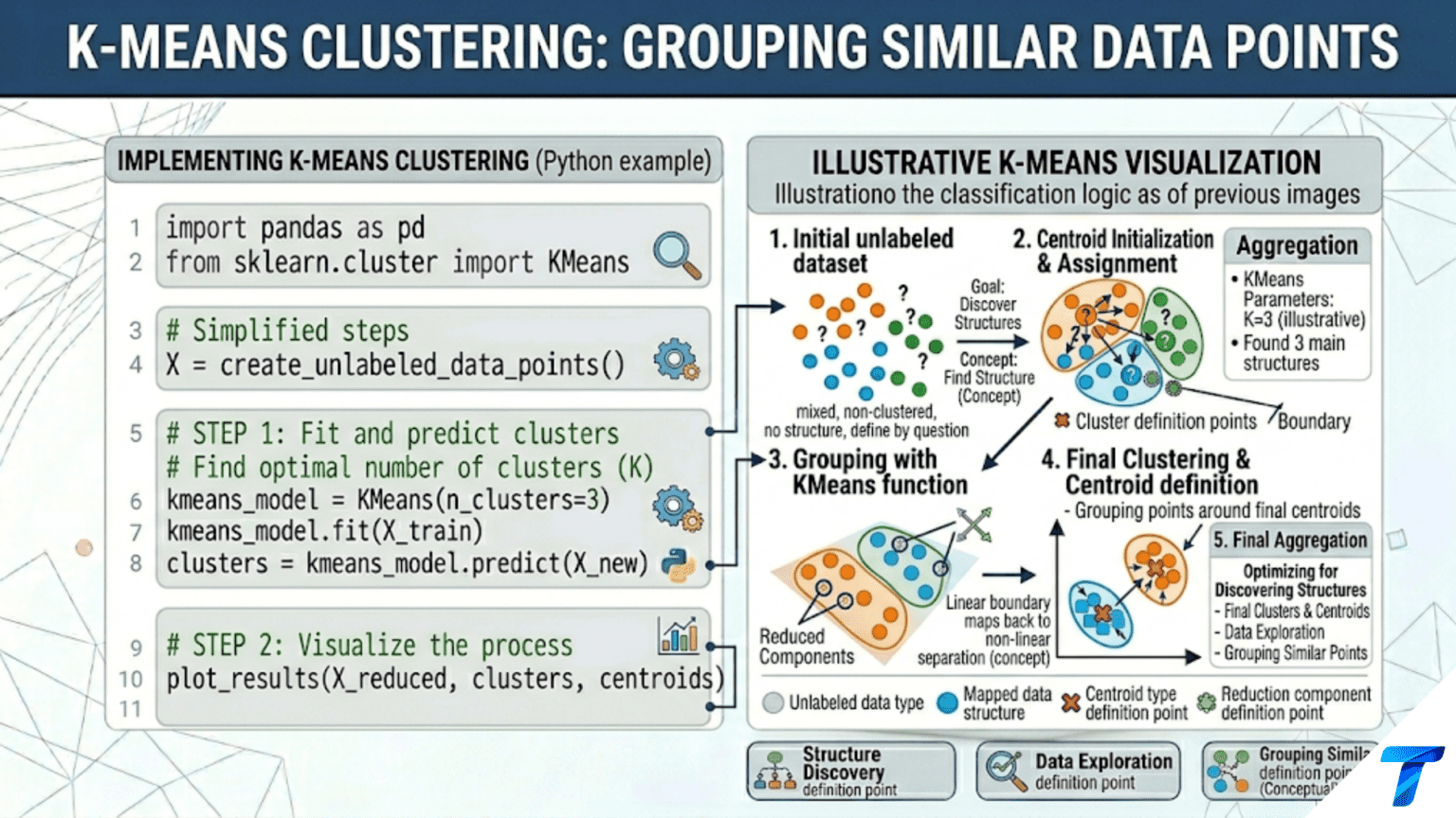
K-Means clustering partitions n data points into k clusters by iterating two steps: (1) assign each point to the nearest centroid, and (2) recompute each centroid as the mean of all points assigned to it. This process repeats until assignments stop changing. The result is k groups where within-cluster points are as similar as possible (small within-cluster variance) and between-cluster points are as different as possible (large between-cluster variance).
Introduction
Imagine you are a marketing analyst with a database of 100,000 customers, each described by a dozen behavioral metrics: purchase frequency, average order value, product categories browsed, days since last purchase, and so on. You want to personalize your email campaigns by segment — but no one has ever defined what the segments are, and you have no historical labels to learn from.
K-Means is the algorithm most commonly applied to exactly this kind of problem. Given a dataset and a number k, it discovers k natural groupings with no human input beyond that single parameter. The algorithm is simple enough to implement from scratch in 30 lines of Python, fast enough to run on millions of points, and interpretable enough that the clusters it discovers can be characterized and named by domain experts.
K-Means is also a rigorous introduction to the core ideas of all clustering: what does it mean for points to be “similar”? How do we measure the quality of a clustering? What assumptions does the algorithm make about the shape of clusters, and when do those assumptions fail? Understanding K-Means deeply is the foundation for understanding every more sophisticated clustering method.
This article builds complete understanding of K-Means: the geometric intuition, the Lloyd’s algorithm, initialization strategies, convergence guarantees, the objective function being minimized, limitations, and practical application with scikit-learn.
The Core Idea: Centroids and Assignments
K-Means organizes data around k centroids — representative points, one per cluster. Every data point belongs to the cluster whose centroid is nearest (measured by Euclidean distance). The key insight is that this assignment-update cycle converges: each iteration of the two steps can only decrease the total within-cluster variance, so the algorithm must eventually reach a fixed point where no more improvements are possible.
import numpy as np
import matplotlib.pyplot as plt
from sklearn.datasets import make_blobs
from sklearn.preprocessing import StandardScaler
import warnings
warnings.filterwarnings('ignore')

np.random.seed(42)


def visualize_kmeans_intuition(figsize=(15, 5)):
    """
    Visual explanation of K-Means: show the before and after.
    Left:  raw unlabeled data (no structure visible to a naive observer)
    Middle: K-Means centroids and Voronoi regions (how the space is partitioned)
    Right:  final cluster assignments with labeled centroids
    """
    from sklearn.cluster import KMeans

    X, y_true = make_blobs(n_samples=250, centers=3, cluster_std=0.8,
                            random_state=42)
    scaler = StandardScaler()
    X_s = scaler.fit_transform(X)

    km = KMeans(n_clusters=3, random_state=42, n_init=10)
    labels = km.fit_predict(X_s)
    centroids = km.cluster_centers_

    fig, axes = plt.subplots(1, 3, figsize=figsize)

    cluster_colors = ['#e74c3c', '#3498db', '#2ecc71']

    # ── Panel 1: Raw unlabeled data ──────────────────────────────
    ax = axes[0]
    ax.scatter(X_s[:, 0], X_s[:, 1], c='steelblue', s=35,
               edgecolors='white', linewidth=0.4, alpha=0.7)
    ax.set_title('Step 0: Raw Unlabeled Data\n'
                 'No structure visible without the algorithm',
                 fontsize=10, fontweight='bold')
    ax.set_xlabel('Feature 1 (scaled)', fontsize=9)
    ax.set_ylabel('Feature 2 (scaled)', fontsize=9)
    ax.grid(True, alpha=0.2)

    # ── Panel 2: Voronoi partition (decision regions) ─────────────
    ax = axes[1]
    x_min, x_max = X_s[:, 0].min() - 0.5, X_s[:, 0].max() + 0.5
    y_min, y_max = X_s[:, 1].min() - 0.5, X_s[:, 1].max() + 0.5
    xx, yy = np.meshgrid(np.linspace(x_min, x_max, 300),
                          np.linspace(y_min, y_max, 300))
    Z = km.predict(np.c_[xx.ravel(), yy.ravel()]).reshape(xx.shape)
    ax.contourf(xx, yy, Z, alpha=0.15,
                colors=cluster_colors[:3])
    ax.contour(xx, yy, Z, colors='gray', linewidths=1.0,
               linestyles='--', alpha=0.5)
    ax.scatter(X_s[:, 0], X_s[:, 1], c='gray', s=20,
               edgecolors='white', linewidth=0.3, alpha=0.5)
    ax.scatter(centroids[:, 0], centroids[:, 1], marker='*',
               s=400, c=cluster_colors[:3], edgecolors='black',
               linewidth=1.5, zorder=5)
    ax.set_title('K-Means Voronoi Partition\n'
                 'Space divided into k regions by nearest centroid',
                 fontsize=10, fontweight='bold')
    ax.set_xlabel('Feature 1 (scaled)', fontsize=9)
    ax.grid(True, alpha=0.2)

    # ── Panel 3: Final cluster assignments ───────────────────────
    ax = axes[2]
    for cls, color in enumerate(cluster_colors[:3]):
        mask = labels == cls
        ax.scatter(X_s[mask, 0], X_s[mask, 1], c=color, s=40,
                   edgecolors='white', linewidth=0.4, alpha=0.85,
                   label=f'Cluster {cls} (n={mask.sum()})')
    ax.scatter(centroids[:, 0], centroids[:, 1], marker='*',
               s=400, c=cluster_colors[:3], edgecolors='black',
               linewidth=1.5, zorder=5, label='Centroids')
    ax.set_title('Final Cluster Assignments\n'
                 'Each point belongs to its nearest centroid',
                 fontsize=10, fontweight='bold')
    ax.set_xlabel('Feature 1 (scaled)', fontsize=9)
    ax.legend(fontsize=8, loc='upper right')
    ax.grid(True, alpha=0.2)

    plt.suptitle('K-Means Clustering: How Space Is Partitioned Into k Groups',
                 fontsize=13, fontweight='bold', y=1.02)
    plt.tight_layout()
    plt.savefig('kmeans_intuition.png', dpi=150, bbox_inches='tight')
    plt.show()
    print("Saved: kmeans_intuition.png")


visualize_kmeans_intuition()Lloyd’s Algorithm: Step-by-Step
The standard K-Means algorithm is formally known as Lloyd’s algorithm (after Stuart Lloyd, who described it in 1957). It alternates between two steps until convergence.
import numpy as np
import matplotlib.pyplot as plt
from sklearn.datasets import make_blobs
from sklearn.preprocessing import StandardScaler


class KMeansFromScratch:
    """
    K-Means clustering implemented from scratch.
    Follows Lloyd's algorithm exactly, tracking every iteration for visualization.
    """

    def __init__(self, k, max_iter=300, tol=1e-4, init='random', random_state=None):
        """
        Args:
            k:            Number of clusters
            max_iter:     Maximum number of E-M iterations
            tol:          Convergence tolerance (centroid movement threshold)
            init:         Initialization strategy: 'random' or 'kmeans++'
            random_state: Seed for reproducibility
        """
        self.k            = k
        self.max_iter     = max_iter
        self.tol          = tol
        self.init         = init
        self.random_state = random_state

        self.centroids_    = None
        self.labels_       = None
        self.inertia_      = None
        self.n_iter_       = 0
        self.history_      = []   # Stores (centroids, labels) at each iteration

    def _init_centroids(self, X):
        """Initialize centroids using either random sampling or K-Means++."""
        rng = np.random.RandomState(self.random_state)
        n, d = X.shape

        if self.init == 'random':
            # Choose k points uniformly at random from the data
            idx = rng.choice(n, size=self.k, replace=False)
            return X[idx].copy()

        elif self.init == 'kmeans++':
            # K-Means++ initialization: choose centroids with probability
            # proportional to squared distance from nearest existing centroid.
            # This spreads the initial centroids and dramatically reduces
            # the chance of poor initializations.
            centroids = [X[rng.randint(n)].copy()]

            for _ in range(1, self.k):
                # Compute distance from each point to its nearest centroid
                dists = np.array([
                    min(np.linalg.norm(x - c) ** 2 for c in centroids)
                    for x in X
                ])
                # Probability proportional to squared distance
                probs = dists / dists.sum()
                cumprobs = np.cumsum(probs)
                r = rng.rand()
                idx = np.searchsorted(cumprobs, r)
                centroids.append(X[idx].copy())

            return np.array(centroids)
        else:
            raise ValueError(f"Unknown init method: {self.init}")

    def _assign_labels(self, X):
        """
        E-step: assign each point to the nearest centroid.
        Returns integer label array of shape (n_samples,).
        """
        # Compute squared Euclidean distance from every point to every centroid
        # Shape: (n_samples, k)
        diffs = X[:, np.newaxis, :] - self.centroids_[np.newaxis, :, :]
        sq_dists = np.sum(diffs ** 2, axis=2)
        return np.argmin(sq_dists, axis=1)

    def _update_centroids(self, X, labels):
        """
        M-step: recompute each centroid as the mean of its assigned points.
        Returns new centroid array of shape (k, n_features).
        """
        new_centroids = np.zeros_like(self.centroids_)
        for cls in range(self.k):
            mask = labels == cls
            if mask.sum() > 0:
                new_centroids[cls] = X[mask].mean(axis=0)
            else:
                # Empty cluster: reinitialize randomly (rare edge case)
                rng = np.random.RandomState(self.random_state)
                new_centroids[cls] = X[rng.randint(len(X))]
        return new_centroids

    def _compute_inertia(self, X, labels):
        """
        Within-cluster sum of squared distances (WCSS).
        This is the objective function K-Means minimizes.
        Lower = better.
        """
        total = 0.0
        for cls in range(self.k):
            mask = labels == cls
            if mask.sum() > 0:
                diffs = X[mask] - self.centroids_[cls]
                total += np.sum(diffs ** 2)
        return total

    def fit(self, X):
        """
        Run Lloyd's algorithm until convergence or max_iter.
        """
        X = np.array(X, dtype=float)

        # Initialize centroids
        self.centroids_ = self._init_centroids(X)

        for iteration in range(self.max_iter):
            # E-step: assign labels
            labels = self._assign_labels(X)

            # Save history for visualization
            self.history_.append({
                'iter':      iteration,
                'centroids': self.centroids_.copy(),
                'labels':    labels.copy(),
                'inertia':   self._compute_inertia(X, labels),
            })

            # M-step: update centroids
            new_centroids = self._update_centroids(X, labels)

            # Check convergence: maximum centroid movement
            centroid_shift = np.max(
                np.linalg.norm(new_centroids - self.centroids_, axis=1)
            )
            self.centroids_ = new_centroids
            self.n_iter_    = iteration + 1

            if centroid_shift < self.tol:
                break

        # Final assignment and inertia
        self.labels_  = self._assign_labels(X)
        self.inertia_ = self._compute_inertia(X, self.labels_)
        return self

    def predict(self, X):
        """Assign new points to the nearest centroid."""
        X = np.array(X, dtype=float)
        return self._assign_labels(X)

    def fit_predict(self, X):
        return self.fit(X).labels_


# Demonstrate the algorithm step by step
print("=== Lloyd's Algorithm: Iteration-by-Iteration ===\n")

np.random.seed(42)
X_demo, _ = make_blobs(n_samples=150, centers=3, cluster_std=0.7,
                        random_state=42)
X_demo_s = StandardScaler().fit_transform(X_demo)

km_scratch = KMeansFromScratch(k=3, init='kmeans++', random_state=42)
km_scratch.fit(X_demo_s)

print(f"  Converged in {km_scratch.n_iter_} iterations\n")
print(f"  {'Iter':>5} | {'Inertia':>12} | {'Change':>12} | Status")
print("  " + "-" * 48)

prev_inertia = None
for step in km_scratch.history_:
    change = (f"{step['inertia'] - prev_inertia:+.4f}"
              if prev_inertia is not None else "     —")
    status = "Converged" if step['iter'] == km_scratch.n_iter_ - 1 else "→"
    print(f"  {step['iter']+1:>5} | {step['inertia']:>12.4f} | {change:>12} | {status}")
    prev_inertia = step['inertia']

print(f"\n  Final inertia: {km_scratch.inertia_:.4f}")
print(f" Inertia ALWAYS decreases with each iteration (guaranteed)")Visualizing the Convergence
import numpy as np
import matplotlib.pyplot as plt
from sklearn.datasets import make_blobs
from sklearn.preprocessing import StandardScaler


def animate_kmeans_convergence(X_s, km_scratch, max_steps=6, figsize=(18, 8)):
    """
    Show the first few iterations of K-Means convergence visually.
    Each subplot shows one iteration: current centroids and new assignments.
    """
    n_show   = min(max_steps, len(km_scratch.history_))
    n_cols   = min(n_show, 3)
    n_rows   = int(np.ceil(n_show / n_cols))
    fig, axes = plt.subplots(n_rows, n_cols,
                              figsize=(6 * n_cols, 5 * n_rows))
    axes = np.array(axes).flatten()

    cluster_colors = ['#e74c3c', '#3498db', '#2ecc71']
    marker_styles  = ['o', 's', 'D']

    for step_i, step in enumerate(km_scratch.history_[:n_show]):
        ax = axes[step_i]
        centroids = step['centroids']
        labels    = step['labels']
        inertia   = step['inertia']

        # Points colored by current cluster assignment
        for cls, color in enumerate(cluster_colors):
            mask = labels == cls
            ax.scatter(X_s[mask, 0], X_s[mask, 1], c=color, s=30,
                       edgecolors='white', linewidth=0.4, alpha=0.75,
                       marker=marker_styles[cls])

        # Centroids
        ax.scatter(centroids[:, 0], centroids[:, 1],
                   marker='*', s=350,
                   c=cluster_colors[:len(centroids)],
                   edgecolors='black', linewidth=1.5, zorder=5)

        # Draw lines from centroids to show movement (after first step)
        if step_i > 0:
            prev_centroids = km_scratch.history_[step_i - 1]['centroids']
            for j in range(len(centroids)):
                ax.annotate('', xy=centroids[j],
                            xytext=prev_centroids[j],
                            arrowprops=dict(arrowstyle='->', color='black',
                                            lw=1.5, alpha=0.6))

        convergence_note = ""
        if step_i == len(km_scratch.history_) - 1:
            convergence_note = "\n✓ Converged"

        ax.set_title(f'Iteration {step["iter"] + 1}\n'
                     f'Inertia = {inertia:.3f}{convergence_note}',
                     fontsize=10, fontweight='bold')
        ax.set_xlabel('Feature 1', fontsize=9)
        if step_i % n_cols == 0:
            ax.set_ylabel('Feature 2', fontsize=9)
        ax.grid(True, alpha=0.2)

    for ax in axes[n_show:]:
        ax.set_visible(False)

    plt.suptitle("K-Means Lloyd's Algorithm: Convergence Animation\n"
                 "(Arrows show centroid movement between iterations)",
                 fontsize=13, fontweight='bold')
    plt.tight_layout()
    plt.savefig('kmeans_convergence.png', dpi=150, bbox_inches='tight')
    plt.show()
    print("Saved: kmeans_convergence.png")


np.random.seed(42)
X_anim, _ = make_blobs(n_samples=150, centers=3, cluster_std=0.7, random_state=42)
X_anim_s  = StandardScaler().fit_transform(X_anim)

km_anim = KMeansFromScratch(k=3, init='random', random_state=7)
km_anim.fit(X_anim_s)

animate_kmeans_convergence(X_anim_s, km_anim, max_steps=6)The Objective Function: Within-Cluster Sum of Squares
K-Means minimizes the Within-Cluster Sum of Squares (WCSS), also called inertia:
where μ_j is the centroid of cluster C_j. This is the total squared distance from every point to its assigned centroid. Every step of Lloyd’s algorithm is guaranteed to either decrease WCSS or leave it unchanged — this is why the algorithm always converges (though not necessarily to the global minimum).
The proof is simple: in the E-step, reassigning a point to a nearer centroid can only decrease WCSS. In the M-step, the mean minimizes the sum of squared deviations from any other point. Therefore each full iteration is a non-increasing step on the WCSS surface.
import numpy as np
import matplotlib.pyplot as plt
from sklearn.datasets import make_blobs
from sklearn.preprocessing import StandardScaler


def visualize_wcss_landscape(X_s, k=3, n_runs=20, figsize=(14, 5)):
    """
    Show WCSS across multiple runs with different initializations.

    K-Means finds a LOCAL minimum, not necessarily the global minimum.
    Different initializations lead to different local minima.
    K-Means++ (default in sklearn) dramatically improves initialization.
    """
    wcss_random  = []
    wcss_kmeanspp = []

    for seed in range(n_runs):
        km_r = KMeansFromScratch(k=k, init='random',   random_state=seed)
        km_p = KMeansFromScratch(k=k, init='kmeans++', random_state=seed)
        km_r.fit(X_s)
        km_p.fit(X_s)
        wcss_random.append(km_r.inertia_)
        wcss_kmeanspp.append(km_p.inertia_)

    fig, axes = plt.subplots(1, 2, figsize=figsize)

    # Distribution of final WCSS across runs
    ax = axes[0]
    ax.hist(wcss_random,  bins=12, alpha=0.7, color='coral',
            label='Random init', edgecolor='white')
    ax.hist(wcss_kmeanspp, bins=12, alpha=0.7, color='steelblue',
            label='K-Means++ init', edgecolor='white')
    ax.axvline(min(wcss_random),   color='coral',
               linestyle='--', lw=2, label=f'Best random: {min(wcss_random):.2f}')
    ax.axvline(min(wcss_kmeanspp), color='steelblue',
               linestyle='--', lw=2, label=f'Best K-Means++: {min(wcss_kmeanspp):.2f}')
    ax.set_xlabel('Final WCSS (inertia)', fontsize=11)
    ax.set_ylabel('Count across runs', fontsize=11)
    ax.set_title(f'WCSS Distribution over {n_runs} Random Initializations\n'
                 f'K-Means++ avoids the worst local minima',
                 fontsize=10, fontweight='bold')
    ax.legend(fontsize=8); ax.grid(True, alpha=0.3)

    # Convergence speed comparison
    ax = axes[1]
    # Pick one typical run of each
    km_r_ex  = KMeansFromScratch(k=k, init='random',   random_state=0)
    km_pp_ex = KMeansFromScratch(k=k, init='kmeans++', random_state=0)
    km_r_ex.fit(X_s); km_pp_ex.fit(X_s)

    iters_r  = [s['inertia'] for s in km_r_ex.history_]
    iters_pp = [s['inertia'] for s in km_pp_ex.history_]

    ax.plot(range(1, len(iters_r)  + 1), iters_r,  'o-', color='coral',
            lw=2.5, markersize=6, label=f'Random ({km_r_ex.n_iter_} iters)')
    ax.plot(range(1, len(iters_pp) + 1), iters_pp, 's-', color='steelblue',
            lw=2.5, markersize=6, label=f'K-Means++ ({km_pp_ex.n_iter_} iters)')
    ax.set_xlabel('Iteration', fontsize=11)
    ax.set_ylabel('WCSS (inertia)', fontsize=11)
    ax.set_title('Convergence Speed: Random vs K-Means++\n'
                 'K-Means++ starts closer to optimum → fewer iterations',
                 fontsize=10, fontweight='bold')
    ax.legend(fontsize=9); ax.grid(True, alpha=0.3)

    plt.suptitle('K-Means Local Minima Problem and K-Means++ Solution',
                 fontsize=13, fontweight='bold')
    plt.tight_layout()
    plt.savefig('kmeans_wcss_landscape.png', dpi=150)
    plt.show()
    print("Saved: kmeans_wcss_landscape.png")

    print(f"\n  Random init:   WCSS range [{min(wcss_random):.2f}, "
          f"{max(wcss_random):.2f}] — "
          f"spread = {max(wcss_random) - min(wcss_random):.2f}")
    print(f"  K-Means++ init: WCSS range [{min(wcss_kmeanspp):.2f}, "
          f"{max(wcss_kmeanspp):.2f}] — "
          f"spread = {max(wcss_kmeanspp) - min(wcss_kmeanspp):.2f}")
    print(f"\n  K-Means++ reduces variance across runs and finds better solutions.")


np.random.seed(42)
X_wcss, _ = make_blobs(n_samples=200, centers=3, cluster_std=0.8,
                        random_state=42)
X_wcss_s  = StandardScaler().fit_transform(X_wcss)
visualize_wcss_landscape(X_wcss_s)K-Means++ Initialization: Why It Matters
Random initialization is unreliable — it can place multiple initial centroids in the same cluster, leaving other clusters uncovered. K-Means++ (Arthur & Vassilvitskii, 2007) uses a smarter initialization: after choosing the first centroid randomly, each subsequent centroid is chosen with probability proportional to its squared distance from the nearest already-chosen centroid. This spreads the initial centroids across the data, avoiding the worst local minima.
K-Means++ provides a theoretical guarantee: the expected WCSS of the K-Means++ initialization is O(log k) times the optimal WCSS. In practice it typically finds solutions within a few percent of optimal, often in fewer iterations than random initialization.
Scikit-learn uses K-Means++ by default (init='k-means++') and runs multiple initializations (n_init=10), keeping the best result.
import numpy as np
from sklearn.cluster import KMeans
from sklearn.datasets import make_blobs
from sklearn.preprocessing import StandardScaler
from sklearn.metrics import silhouette_score
import time


def compare_init_strategies(X_s, k=3, n_runs=50):
    """
    Quantitative comparison of initialization strategies.
    """
    print("=== Initialization Strategy Comparison ===\n")
    print(f"  k={k}, {n_runs} independent runs per strategy\n")
    print(f"  {'Strategy':<20} | {'Mean WCSS':>12} | {'Std WCSS':>10} | "
          f"{'Best WCSS':>11} | {'Mean iters':>11} | {'Time (s)':>9}")
    print("  " + "-" * 80)

    strategies = {
        'random (n_init=1)':    {'init': 'random',    'n_init': 1},
        'random (n_init=10)':   {'init': 'random',    'n_init': 10},
        'k-means++ (n_init=1)': {'init': 'k-means++', 'n_init': 1},
        'k-means++ (n_init=10)':{'init': 'k-means++', 'n_init': 10},
    }

    for name, params in strategies.items():
        wcss_vals = []
        iter_vals = []
        t_start   = time.perf_counter()

        for seed in range(n_runs):
            km = KMeans(n_clusters=k, **params, random_state=seed)
            km.fit(X_s)
            wcss_vals.append(km.inertia_)
            iter_vals.append(km.n_iter_)

        elapsed = time.perf_counter() - t_start

        print(f"  {name:<20} | {np.mean(wcss_vals):>12.4f} | "
              f"{np.std(wcss_vals):>10.4f} | {min(wcss_vals):>11.4f} | "
              f"{np.mean(iter_vals):>11.1f} | {elapsed:>9.3f}")

    print(f"\n  Recommendation: Use default 'k-means++' with n_init=10.")
    print(f"  For large datasets, n_init='auto' (sklearn ≥ 1.2) is efficient.")


np.random.seed(42)
X_init, _ = make_blobs(n_samples=300, centers=4, cluster_std=0.8, random_state=42)
X_init_s  = StandardScaler().fit_transform(X_init)
compare_init_strategies(X_init_s, k=4)K-Means with Scikit-Learn: Production Usage
import numpy as np
import matplotlib.pyplot as plt
from sklearn.cluster import KMeans
from sklearn.datasets import make_blobs, load_digits
from sklearn.preprocessing import StandardScaler
from sklearn.decomposition import PCA
from sklearn.metrics import silhouette_score, adjusted_rand_score
from sklearn.pipeline import Pipeline


def kmeans_production_pipeline(X, y_true=None, k=3,
                                 dataset_name="Dataset"):
    """
    Production-quality K-Means pipeline with:
    - Mandatory feature scaling
    - K-Means++ initialization
    - Multiple restarts (n_init)
    - Evaluation with silhouette score
    - 2D PCA visualization of results
    """
    print(f"=== K-Means Production Pipeline: {dataset_name} ===\n")
    print(f"  n={len(X)}, d={X.shape[1]}, k={k}\n")

    # Step 1: Scale
    scaler = StandardScaler()
    X_s = scaler.fit_transform(X)

    # Step 2: Fit with best practices
    km = KMeans(
        n_clusters=k,
        init='k-means++',   # Smart initialization
        n_init=20,           # 20 independent runs, keep best
        max_iter=300,        # Enough iterations to converge
        tol=1e-4,            # Convergence threshold
        random_state=42,
        algorithm='lloyd',   # Standard Lloyd's algorithm
    )
    labels = km.fit_predict(X_s)

    # Step 3: Evaluate
    sil = silhouette_score(X_s, labels)
    inertia = km.inertia_
    n_iter  = km.n_iter_

    print(f"  Results:")
    print(f"    Inertia (WCSS):   {inertia:.4f}")
    print(f"    Silhouette Score: {sil:.4f}  (range [-1,1], higher=better)")
    print(f"    Iterations:       {n_iter}")
    print(f"    n_init runs:      20 (best selected)")

    if y_true is not None:
        ari = adjusted_rand_score(y_true, labels)
        print(f"    ARI vs ground truth: {ari:.4f}")

    # Step 4: Cluster profiles
    print(f"\n  Cluster Profiles:")
    print(f"  {'Cluster':>8} | {'Size':>6} | {'% data':>8} | {'Avg dist to centroid':>22}")
    print("  " + "-" * 50)

    for cls in range(k):
        mask       = labels == cls
        cluster_X  = X_s[mask]
        centroid   = km.cluster_centers_[cls]
        avg_dist   = np.mean(np.linalg.norm(cluster_X - centroid, axis=1))
        pct        = 100 * mask.sum() / len(X)
        print(f"  {cls:>8} | {mask.sum():>6} | {pct:>8.1f}% | {avg_dist:>22.4f}")

    # Step 5: Visualize via PCA
    pca = PCA(n_components=2, random_state=42)
    X_2d = pca.fit_transform(X_s)
    var_explained = pca.explained_variance_ratio_.sum() * 100

    fig, axes = plt.subplots(1, 2, figsize=(13, 5))
    colors = plt.cm.tab10(np.linspace(0, 1, k))

    ax = axes[0]
    for cls, color in enumerate(colors):
        mask = labels == cls
        ax.scatter(X_2d[mask, 0], X_2d[mask, 1], c=[color], s=30,
                   edgecolors='white', linewidth=0.4, alpha=0.8,
                   label=f'Cluster {cls} (n={mask.sum()})')
    centroids_2d = pca.transform(km.cluster_centers_)
    ax.scatter(centroids_2d[:, 0], centroids_2d[:, 1],
               marker='*', s=350, c='black', zorder=5, label='Centroids')
    ax.set_title(f'K-Means Clusters in PCA Space\n'
                 f'({var_explained:.1f}% variance explained by 2 PCs)',
                 fontsize=10, fontweight='bold')
    ax.set_xlabel('PC1', fontsize=9); ax.set_ylabel('PC2', fontsize=9)
    ax.legend(fontsize=7, loc='best'); ax.grid(True, alpha=0.2)

    # Inertia curve (re-run for k=1..10)
    ax = axes[1]
    k_vals  = range(1, 11)
    inertias = []
    for kk in k_vals:
        kmi = KMeans(n_clusters=kk, init='k-means++', n_init=10,
                     random_state=42)
        kmi.fit(X_s)
        inertias.append(kmi.inertia_)

    ax.plot(k_vals, inertias, 'o-', color='steelblue', lw=2.5, markersize=8)
    ax.axvline(x=k, color='coral', linestyle='--', lw=2,
               label=f'Chosen k={k}')
    ax.set_xlabel('k (number of clusters)', fontsize=11)
    ax.set_ylabel('Inertia (WCSS)', fontsize=11)
    ax.set_title('Elbow Curve\n(Inertia vs k — look for the "elbow")',
                 fontsize=10, fontweight='bold')
    ax.legend(fontsize=9); ax.grid(True, alpha=0.3)

    plt.suptitle(f'K-Means: {dataset_name}', fontsize=13, fontweight='bold')
    plt.tight_layout()
    plt.savefig(f'kmeans_production_{dataset_name.lower().replace(" ", "_")}.png',
                dpi=150)
    plt.show()
    print(f"\nSaved: kmeans_production_{dataset_name.lower().replace(' ', '_')}.png")

    return km, labels


np.random.seed(42)
X_prod, y_prod = make_blobs(n_samples=400, centers=4, cluster_std=0.9, random_state=42)
km_result, labels_result = kmeans_production_pipeline(
    X_prod, y_true=y_prod, k=4, dataset_name="Synthetic Blobs"
)K-Means Limitations: When the Algorithm Fails
Understanding when K-Means fails is as important as knowing how to use it. The algorithm’s core assumptions — spherical clusters, equal-size clusters, Euclidean distance — lead to predictable failure modes.
import numpy as np
import matplotlib.pyplot as plt
from sklearn.cluster import KMeans
from sklearn.preprocessing import StandardScaler
from sklearn.datasets import make_moons, make_circles


def demonstrate_kmeans_limitations(figsize=(18, 12)):
    """
    Four canonical failure cases for K-Means:
    1. Non-spherical clusters (moons, rings)
    2. Highly unequal cluster sizes
    3. Highly unequal cluster densities
    4. High-dimensional data with irrelevant features
    """
    np.random.seed(42)
    fig, axes = plt.subplots(2, 2, figsize=figsize)
    axes = axes.flatten()

    scaler = StandardScaler()

    # ── Failure 1: Non-spherical clusters ─────────────────────────
    ax = axes[0]
    X_moons, y_moons = make_moons(n_samples=300, noise=0.1, random_state=42)
    X_m = scaler.fit_transform(X_moons)
    km  = KMeans(n_clusters=2, random_state=42, n_init=10)
    pred = km.fit_predict(X_m)

    from sklearn.metrics import adjusted_rand_score
    ari = adjusted_rand_score(y_moons, pred)

    colors = ['#e74c3c', '#3498db']
    for cls, color in enumerate(colors):
        mask = pred == cls
        ax.scatter(X_m[mask, 0], X_m[mask, 1], c=color, s=25,
                   edgecolors='white', linewidth=0.3, alpha=0.8)
    ax.scatter(km.cluster_centers_[:, 0], km.cluster_centers_[:, 1],
               marker='*', s=300, c='black', zorder=5)
    ax.set_title(f'Failure 1: Non-Spherical Clusters\n'
                 f'True shape: two moons | K-Means ARI = {ari:.3f}\n'
                 '→ Use DBSCAN or Spectral Clustering instead',
                 fontsize=9, fontweight='bold')
    ax.grid(True, alpha=0.2)

    # ── Failure 2: Unequal cluster sizes ──────────────────────────
    ax = axes[1]
    X_unequal = np.vstack([
        np.random.randn(20, 2) * 0.3 + np.array([0, 0]),    # 20 points
        np.random.randn(280, 2) * 0.5 + np.array([3, 0]),   # 280 points
    ])
    y_unequal = np.array([0]*20 + [1]*280)
    X_u = scaler.fit_transform(X_unequal)
    km2 = KMeans(n_clusters=2, random_state=42, n_init=10)
    pred2 = km2.fit_predict(X_u)
    ari2  = adjusted_rand_score(y_unequal, pred2)

    for cls, color in enumerate(colors):
        mask = pred2 == cls
        ax.scatter(X_u[mask, 0], X_u[mask, 1], c=color, s=25,
                   edgecolors='white', linewidth=0.3, alpha=0.8)
    ax.scatter(km2.cluster_centers_[:, 0], km2.cluster_centers_[:, 1],
               marker='*', s=300, c='black', zorder=5)
    ax.set_title(f'Failure 2: Unequal Cluster Sizes\n'
                 f'True: 20 vs 280 | K-Means ARI = {ari2:.3f}\n'
                 '→ K-Means biased toward equal-size clusters',
                 fontsize=9, fontweight='bold')
    ax.grid(True, alpha=0.2)

    # ── Failure 3: Unequal cluster densities ──────────────────────
    ax = axes[2]
    X_dense = np.vstack([
        np.random.randn(150, 2) * 0.2 + np.array([0, 0]),  # Dense cluster
        np.random.randn(150, 2) * 2.0 + np.array([4, 0]),  # Sparse cluster
    ])
    y_dense = np.array([0]*150 + [1]*150)
    X_d = scaler.fit_transform(X_dense)
    km3  = KMeans(n_clusters=2, random_state=42, n_init=10)
    pred3 = km3.fit_predict(X_d)
    ari3  = adjusted_rand_score(y_dense, pred3)

    for cls, color in enumerate(colors):
        mask = pred3 == cls
        ax.scatter(X_d[mask, 0], X_d[mask, 1], c=color, s=25,
                   edgecolors='white', linewidth=0.3, alpha=0.8)
    ax.scatter(km3.cluster_centers_[:, 0], km3.cluster_centers_[:, 1],
               marker='*', s=300, c='black', zorder=5)
    ax.set_title(f'Failure 3: Unequal Cluster Densities\n'
                 f'True: dense vs sparse | K-Means ARI = {ari3:.3f}\n'
                 '→ Dense cluster "bleeds" into sparse region',
                 fontsize=9, fontweight='bold')
    ax.grid(True, alpha=0.2)

    # ── Failure 4: Irrelevant features dominate distance ──────────
    ax = axes[3]
    # Two clusters separated in dimension 0 only; dim 1 is pure noise
    X_irrel = np.column_stack([
        np.concatenate([np.random.randn(150), np.random.randn(150) + 5]),
        np.random.randn(300) * 10  # Large-variance irrelevant feature
    ])
    y_irrel = np.array([0]*150 + [1]*150)
    X_ir = scaler.fit_transform(X_irrel)
    km4   = KMeans(n_clusters=2, random_state=42, n_init=10)
    pred4 = km4.fit_predict(X_ir)
    ari4  = adjusted_rand_score(y_irrel, pred4)

    for cls, color in enumerate(colors):
        mask = pred4 == cls
        ax.scatter(X_ir[mask, 0], X_ir[mask, 1], c=color, s=20,
                   edgecolors='white', linewidth=0.3, alpha=0.8)
    ax.scatter(km4.cluster_centers_[:, 0], km4.cluster_centers_[:, 1],
               marker='*', s=300, c='black', zorder=5)
    ax.set_title(f'Failure 4: Irrelevant High-Variance Feature\n'
                 f'Feature 2 is pure noise | K-Means ARI = {ari4:.3f}\n'
                 '→ Scale ALL features; consider PCA preprocessing',
                 fontsize=9, fontweight='bold')
    ax.set_xlabel('Feature 1 (signal)', fontsize=8)
    ax.set_ylabel('Feature 2 (noise × 10)', fontsize=8)
    ax.grid(True, alpha=0.2)

    plt.suptitle('K-Means Failure Modes: When the Algorithm Breaks\n'
                 '(All cases use scaled data — failures are geometric, not scaling)',
                 fontsize=13, fontweight='bold')
    plt.tight_layout()
    plt.savefig('kmeans_failures.png', dpi=150, bbox_inches='tight')
    plt.show()
    print("Saved: kmeans_failures.png")


demonstrate_kmeans_limitations()Mini-Batch K-Means: Scaling to Large Datasets
Standard K-Means requires computing distances from every training point to every centroid in every iteration. For very large datasets this becomes slow. Mini-Batch K-Means uses random mini-batches instead, approximating the centroid update and reducing time complexity from O(n·k·d·T) to O(b·k·d·T) where b << n is the batch size.
import numpy as np
import time
from sklearn.cluster import KMeans, MiniBatchKMeans
from sklearn.datasets import make_blobs
from sklearn.preprocessing import StandardScaler
from sklearn.metrics import silhouette_score


def compare_kmeans_minibatch(n_samples=50_000, k=5, batch_sizes=None):
    """
    Compare full K-Means vs Mini-Batch K-Means on a large dataset.
    Trades small accuracy loss for large speed gains.
    """
    if batch_sizes is None:
        batch_sizes = [256, 512, 1024, 2048]

    np.random.seed(42)
    X_large, _ = make_blobs(n_samples=n_samples, centers=k, cluster_std=1.0,
                             random_state=42)
    X_s = StandardScaler().fit_transform(X_large)

    print(f"=== K-Means vs Mini-Batch K-Means ===\n")
    print(f"  n={n_samples:,}, k={k}\n")
    print(f"  {'Method':<30} | {'Time (s)':>9} | {'Inertia':>12} | "
          f"{'Silhouette':>11} | Notes")
    print("  " + "-" * 78)

    # Full K-Means
    t0 = time.perf_counter()
    km_full = KMeans(n_clusters=k, init='k-means++', n_init=3,
                     random_state=42, algorithm='lloyd')
    labels_full = km_full.fit_predict(X_s)
    t_full = time.perf_counter() - t0
    sil_full = silhouette_score(X_s, labels_full, sample_size=5000)

    print(f"  {'Full K-Means':<30} | {t_full:>9.3f} | {km_full.inertia_:>12.1f} | "
          f"{sil_full:>11.4f} | Baseline")

    # Mini-Batch K-Means with various batch sizes
    for batch_size in batch_sizes:
        t0 = time.perf_counter()
        km_mb = MiniBatchKMeans(n_clusters=k, init='k-means++', n_init=3,
                                 batch_size=batch_size, random_state=42,
                                 max_iter=100)
        labels_mb = km_mb.fit_predict(X_s)
        t_mb = time.perf_counter() - t0
        sil_mb = silhouette_score(X_s, labels_mb, sample_size=5000)
        speedup = t_full / t_mb

        inertia_diff_pct = (km_mb.inertia_ - km_full.inertia_) / km_full.inertia_ * 100

        print(f"  {'MiniBatch (b=' + str(batch_size) + ')':<30} | "
              f"{t_mb:>9.3f} | {km_mb.inertia_:>12.1f} | "
              f"{sil_mb:>11.4f} | "
              f"{speedup:.1f}× faster, "
              f"+{inertia_diff_pct:.1f}% inertia")

    print(f"\n  Mini-Batch K-Means trades ~1-5% inertia accuracy for 5-20× speedup.")
    print(f"  For n > 10,000, Mini-Batch is the practical default.")


compare_kmeans_minibatch(n_samples=50_000)K-Means for Image Compression: A Concrete Application
Image compression is one of the most vivid demonstrations of K-Means in action. An image with millions of unique pixel colors can be approximated using only k representative colors — one per cluster. Each pixel is replaced by its nearest centroid color, and the image is stored as k RGB values plus an index per pixel instead of three bytes per pixel.
import numpy as np
import matplotlib.pyplot as plt
from sklearn.cluster import KMeans
from sklearn.utils import shuffle


def compress_image_with_kmeans(n_colors_list=None, figsize=(18, 10)):
    """
    Demonstrate K-Means image compression by reducing a sample image
    from thousands of unique colors to k representative colors.

    Each pixel is replaced by its nearest centroid color.
    Storage: k × 3 bytes (palette) + n × log2(k) bits (indices)
    vs original: n × 3 bytes (one byte per channel per pixel)
    """
    if n_colors_list is None:
        n_colors_list = [2, 4, 8, 16, 64, 256]

    # Create a synthetic colorful image (since we can't load files here)
    np.random.seed(42)
    h, w = 100, 100

    # Create a gradient image with 4 color regions
    image = np.zeros((h, w, 3), dtype=np.float32)
    # Top-left: red-ish
    image[:50, :50] = [0.9, 0.2, 0.2] + np.random.randn(50, 50, 3) * 0.1
    # Top-right: blue-ish
    image[:50, 50:] = [0.2, 0.3, 0.9] + np.random.randn(50, 50, 3) * 0.1
    # Bottom-left: green-ish
    image[50:, :50] = [0.2, 0.8, 0.3] + np.random.randn(50, 50, 3) * 0.1
    # Bottom-right: yellow-ish
    image[50:, 50:] = [0.9, 0.8, 0.1] + np.random.randn(50, 50, 3) * 0.1
    image = np.clip(image, 0, 1)

    # Flatten to (n_pixels, 3) for clustering
    pixels = image.reshape(-1, 3)
    n_unique_colors = len(np.unique(pixels.reshape(-1, 3), axis=0))

    print(f"=== K-Means Image Compression ===\n")
    print(f"  Image: {h}×{w} pixels = {h*w:,} pixels")
    print(f"  Original unique colors: ~{n_unique_colors:,}")
    print(f"  Original storage: {h*w*3:,} bytes (3 channels × 1 byte each)\n")

    n_cols = len(n_colors_list) + 1
    fig, axes = plt.subplots(2, (n_cols + 1) // 2, figsize=figsize)
    axes = axes.flatten()

    # Original image
    axes[0].imshow(image)
    axes[0].set_title(f'Original\n{n_unique_colors} unique colors',
                      fontsize=10, fontweight='bold')
    axes[0].axis('off')

    print(f"  {'k colors':>10} | {'Compression':>12} | {'MSE':>10} | "
          f"{'PSNR (dB)':>11} | Notes")
    print("  " + "-" * 60)

    for ax, k in zip(axes[1:], n_colors_list):
        # Cluster pixel colors into k groups
        km = KMeans(n_clusters=k, init='k-means++', n_init=3,
                    random_state=42)
        km.fit(pixels)

        # Replace each pixel with its cluster's centroid color
        labels   = km.predict(pixels)
        palette  = km.cluster_centers_
        compressed_pixels = palette[labels]
        compressed_image  = compressed_pixels.reshape(h, w, 3)
        compressed_image  = np.clip(compressed_image, 0, 1)

        # Quality metrics
        mse  = np.mean((image - compressed_image) ** 2)
        psnr = 10 * np.log10(1.0 / mse) if mse > 0 else float('inf')

        # Compression ratio
        original_bytes   = h * w * 3
        compressed_bytes = k * 3 + h * w * np.ceil(np.log2(k + 1) / 8)
        ratio = original_bytes / compressed_bytes

        ax.imshow(compressed_image)
        ax.set_title(f'k = {k} colors\nPSNR = {psnr:.1f} dB',
                     fontsize=9, fontweight='bold')
        ax.axis('off')

        quality = ("Poor" if psnr < 25 else
                   ("Acceptable" if psnr < 35 else "Good"))
        print(f"  {k:>10} | {ratio:>11.1f}× | {mse:>10.5f} | "
              f"{psnr:>10.1f} | {quality}")

    for ax in axes[len(n_colors_list) + 1:]:
        ax.set_visible(False)

    plt.suptitle('K-Means Image Compression: Trading Colors for Storage\n'
                 '(Each pixel replaced by its cluster centroid color)',
                 fontsize=13, fontweight='bold')
    plt.tight_layout()
    plt.savefig('kmeans_image_compression.png', dpi=150, bbox_inches='tight')
    plt.show()
    print("\nSaved: kmeans_image_compression.png")
    print("\n  Key insight: With k=64 colors, the image is nearly indistinguishable")
    print("  from the original but requires far less storage.")


compress_image_with_kmeans()K-Means for Customer Segmentation: End-to-End Example
import numpy as np
import matplotlib.pyplot as plt
from sklearn.cluster import KMeans
from sklearn.preprocessing import StandardScaler
from sklearn.decomposition import PCA
from sklearn.metrics import silhouette_score


def customer_segmentation_example(n_customers=800, random_state=42):
    """
    End-to-end customer segmentation with K-Means.

    Features: recency (days since last purchase), frequency (purchases per month),
    monetary (average order value), age, and category preferences.
    This is a simplified version of the classic RFM segmentation model.
    """
    np.random.seed(random_state)

    # Simulate realistic customer data with 4 natural segments
    segment_specs = {
        'Champions':        {'n': 200, 'rec': (5, 3),   'freq': (12, 2),
                              'mon': (250, 60), 'age': (32, 6)},
        'Loyal Customers':  {'n': 250, 'rec': (20, 8),  'freq': (6, 2),
                              'mon': (120, 30), 'age': (38, 9)},
        'At Risk':          {'n': 200, 'rec': (90, 20), 'freq': (2, 1),
                              'mon': (80, 25),  'age': (45, 12)},
        'Lost Customers':   {'n': 150, 'rec': (200, 40),'freq': (0.5, 0.3),
                              'mon': (40, 15),  'age': (52, 10)},
    }

    rows, true_labels, label_names = [], [], []
    for i, (name, spec) in enumerate(segment_specs.items()):
        n = spec['n']
        rec  = np.abs(np.random.normal(spec['rec'][0],  spec['rec'][1],  n))
        freq = np.abs(np.random.normal(spec['freq'][0], spec['freq'][1], n))
        mon  = np.abs(np.random.normal(spec['mon'][0],  spec['mon'][1],  n))
        age  = np.abs(np.random.normal(spec['age'][0],  spec['age'][1],  n))
        rows.append(np.column_stack([rec, freq, mon, age]))
        true_labels.extend([i] * n)
        label_names.extend([name] * n)

    X = np.vstack(rows)
    y_true = np.array(true_labels)
    feature_names = ['Recency (days)', 'Frequency (per month)',
                     'Monetary (avg $)', 'Age']

    # Pipeline
    scaler = StandardScaler()
    X_s = scaler.fit_transform(X)

    # Find best k using silhouette
    sil_scores = []
    k_range = range(2, 9)
    for k in k_range:
        km = KMeans(n_clusters=k, init='k-means++', n_init=10, random_state=42)
        labels = km.fit_predict(X_s)
        sil_scores.append(silhouette_score(X_s, labels))

    best_k = k_range[np.argmax(sil_scores)]

    # Final clustering
    km_final = KMeans(n_clusters=best_k, init='k-means++', n_init=10,
                      random_state=42)
    labels_final = km_final.fit_predict(X_s)

    from sklearn.metrics import adjusted_rand_score
    ari = adjusted_rand_score(y_true, labels_final)

    print(f"=== Customer Segmentation: {n_customers} customers ===\n")
    print(f"  Features: {feature_names}\n")
    print(f"  Best k (by silhouette): {best_k}")
    print(f"  ARI vs true segments:   {ari:.4f}\n")

    # Profile each discovered cluster
    print("  Discovered Cluster Profiles:\n")
    header = (f"  {'Cluster':>8} | {'n':>5} | {'Recency':>9} | "
              f"{'Frequency':>11} | {'Monetary':>10} | {'Age':>6} | Likely Segment")
    print(header)
    print("  " + "-" * 80)

    centroids_unscaled = scaler.inverse_transform(km_final.cluster_centers_)
    for cls in range(best_k):
        mask = labels_final == cls
        c    = centroids_unscaled[cls]
        # Heuristic labeling based on centroid values
        if c[0] < 30 and c[1] > 8:
            seg = "Champions"
        elif c[0] < 50 and c[1] > 4:
            seg = "Loyal Customers"
        elif c[0] < 120:
            seg = "At Risk"
        else:
            seg = "Lost Customers"
        print(f"  {cls:>8} | {mask.sum():>5} | {c[0]:>9.1f} | "
              f"{c[1]:>11.2f} | ${c[2]:>9.0f} | {c[3]:>6.0f} | {seg}")

    # Visualization: PCA + silhouette
    fig, axes = plt.subplots(1, 2, figsize=(13, 5))
    pca = PCA(n_components=2, random_state=42)
    X_2d = pca.fit_transform(X_s)

    ax = axes[0]
    cmap = plt.cm.tab10(np.linspace(0, 0.9, best_k))
    segment_names = list(segment_specs.keys())
    for cls, color in enumerate(cmap):
        mask = labels_final == cls
        ax.scatter(X_2d[mask, 0], X_2d[mask, 1], c=[color],
                   s=25, edgecolors='white', linewidth=0.3, alpha=0.8,
                   label=f'Cluster {cls} (n={mask.sum()})')
    centroids_2d = pca.transform(km_final.cluster_centers_)
    ax.scatter(centroids_2d[:, 0], centroids_2d[:, 1], marker='*',
               s=350, c='black', zorder=5)
    ax.set_title(f'Customer Segments (PCA 2D)\nk={best_k}, ARI={ari:.3f}',
                 fontsize=11, fontweight='bold')
    ax.set_xlabel(f'PC1 ({pca.explained_variance_ratio_[0]*100:.1f}%)', fontsize=9)
    ax.set_ylabel(f'PC2 ({pca.explained_variance_ratio_[1]*100:.1f}%)', fontsize=9)
    ax.legend(fontsize=8); ax.grid(True, alpha=0.2)

    ax = axes[1]
    ax.plot(list(k_range), sil_scores, 'o-', color='steelblue',
            lw=2.5, markersize=9)
    ax.axvline(x=best_k, color='coral', linestyle='--', lw=2,
               label=f'Best k={best_k}')
    ax.set_xlabel('k (number of clusters)', fontsize=11)
    ax.set_ylabel('Silhouette Score', fontsize=11)
    ax.set_title('Silhouette Score vs k\n(Higher = better-defined clusters)',
                 fontsize=11, fontweight='bold')
    ax.legend(fontsize=10); ax.grid(True, alpha=0.3)

    plt.suptitle('K-Means Customer Segmentation: RFM Analysis',
                 fontsize=13, fontweight='bold')
    plt.tight_layout()
    plt.savefig('kmeans_customer_segmentation.png', dpi=150)
    plt.show()
    print("\nSaved: kmeans_customer_segmentation.png")


customer_segmentation_example()Summary
K-Means is the most widely used clustering algorithm because it is fast, simple, and effective when data genuinely clusters into compact spherical groups. Lloyd’s algorithm alternates two steps — assign each point to the nearest centroid, then recompute each centroid as the mean — until convergence. This process is guaranteed to decrease the within-cluster sum of squares (WCSS) monotonically, converging to a local minimum in a finite number of iterations.
The most important practical decisions in applying K-Means are: always scale features before clustering (unscaled features with different ranges dominate the distance calculation); use K-Means++ initialization (reduces sensitivity to initialization and finds better local minima); choose k systematically using the elbow method or silhouette score (covered in article 84); and validate cluster quality with internal metrics like silhouette score rather than trusting the algorithm blindly.
K-Means makes strong geometric assumptions — clusters should be spherical, roughly equal-sized, and of similar density. When these assumptions fail, the algorithm produces misleading results. Non-spherical clusters, extremely unequal sizes, and varying densities all break K-Means in predictable ways. Articles 85 (Hierarchical Clustering) and 86 (DBSCAN) present alternatives that relax these assumptions.
For large datasets (n > 10,000), Mini-Batch K-Means provides near-identical clustering quality with dramatically reduced runtime by updating centroids on random batches rather than the full dataset.