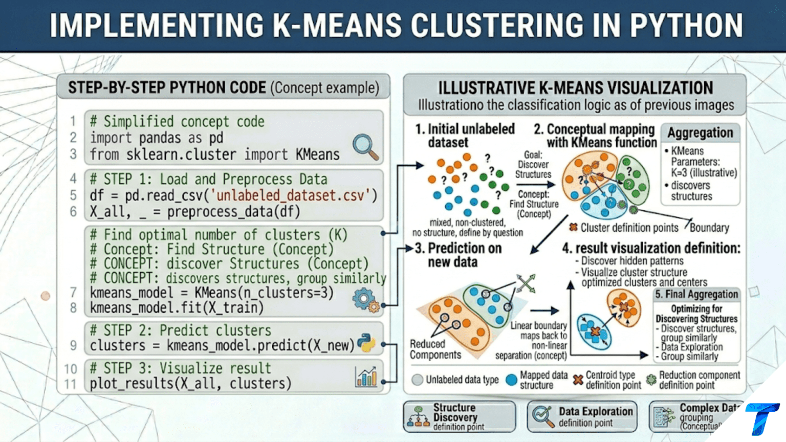
Implementing K-Means in Python requires four steps: (1) scale your features with StandardScaler so no single feature dominates the distance calculation, (2) fit KMeans(n_clusters=k, init='k-means++', n_init=10) from scikit-learn, (3) evaluate quality with silhouette_score, and (4) visualize clusters using PCA to reduce to 2D. The most common mistake is skipping the scaling step — unscaled features with large ranges will dominate the clustering result regardless of their actual relevance.
Introduction
Article 82 explained the theory behind K-Means: Lloyd’s algorithm, the WCSS objective, K-Means++ initialization, and the algorithm’s geometric assumptions. This article is the hands-on companion: how to implement K-Means correctly on real data, step by step.
“Implementing” K-Means means much more than calling KMeans().fit(X). It means making deliberate decisions at every stage: which features to include and how to prepare them, how to choose k, how to evaluate whether the discovered clusters are meaningful, how to profile and visualize the results, how to handle edge cases (empty clusters, very large datasets, high-dimensional data), and how to package the pipeline for production use.
This article covers the complete implementation workflow across multiple real datasets: structured numerical data, text data, and image data. Each dataset illustrates different preprocessing challenges and evaluation strategies. By the end, you will have a reusable K-Means implementation pattern that applies to new problems with minimal modification.
Setup and Imports
import numpy as np
import pandas as pd
import matplotlib.pyplot as plt
import matplotlib.gridspec as gridspec
from sklearn.cluster import KMeans, MiniBatchKMeans
from sklearn.preprocessing import StandardScaler, MinMaxScaler
from sklearn.decomposition import PCA
from sklearn.metrics import (silhouette_score, silhouette_samples,
                              adjusted_rand_score, calinski_harabasz_score,
                              davies_bouldin_score)
from sklearn.datasets import (load_iris, load_wine, load_breast_cancer,
                               make_blobs, make_moons)
from sklearn.pipeline import Pipeline
import warnings
warnings.filterwarnings('ignore')

np.random.seed(42)
print("All imports successful.")
print(f"NumPy: {np.__version__}")
import sklearn; print(f"Scikit-learn: {sklearn.__version__}")Step 1: Data Preparation
The single most important preprocessing step for K-Means is feature scaling. Because K-Means uses Euclidean distance, features with larger numerical ranges dominate the distance calculation — a feature measured in thousands will overshadow a feature measured in fractions, regardless of their actual predictive relevance.
import numpy as np
import pandas as pd
from sklearn.datasets import load_wine
from sklearn.preprocessing import StandardScaler, MinMaxScaler, RobustScaler
from sklearn.cluster import KMeans
from sklearn.metrics import silhouette_score


def compare_scaling_strategies():
    """
    Demonstrate how different scaling strategies affect K-Means clustering.
    Shows that StandardScaler is usually the right default.

    Strategies compared:
    1. No scaling (raw features)
    2. StandardScaler (zero mean, unit variance)
    3. MinMaxScaler (all features in [0, 1])
    4. RobustScaler (uses median and IQR — robust to outliers)
    """
    wine = load_wine()
    X, y_true = wine.data, wine.target
    k = 3  # Wine has 3 true cultivar classes

    print("=== Feature Scaling Impact on K-Means ===\n")
    print(f"  Dataset: Wine ({X.shape[0]} samples, {X.shape[1]} features, k={k})\n")

    # Show feature ranges before scaling
    ranges = X.max(axis=0) - X.min(axis=0)
    print(f"  Feature range spread (max - min):")
    print(f"    Min range: {ranges.min():.4f}  ({wine.feature_names[ranges.argmin()]})")
    print(f"    Max range: {ranges.max():.4f}  ({wine.feature_names[ranges.argmax()]})")
    print(f"    Ratio: {ranges.max() / ranges.min():.1f}× — "
          f"large range dominates without scaling\n")

    scalers = {
        'No scaling':    None,
        'StandardScaler': StandardScaler(),
        'MinMaxScaler':  MinMaxScaler(),
        'RobustScaler':  RobustScaler(),
    }

    print(f"  {'Scaler':<18} | {'Silhouette':>11} | {'ARI':>8} | "
          f"{'CH Score':>10} | {'DB Score':>10}")
    print("  " + "-" * 64)

    best_sil = -1
    best_name = ""

    for name, scaler in scalers.items():
        X_proc = scaler.fit_transform(X) if scaler is not None else X.copy()
        km = KMeans(n_clusters=k, init='k-means++', n_init=20, random_state=42)
        labels = km.fit_predict(X_proc)

        sil = silhouette_score(X_proc, labels)
        ari = adjusted_rand_score(y_true, labels)
        ch  = calinski_harabasz_score(X_proc, labels)
        db  = davies_bouldin_score(X_proc, labels)

        flag = " ← best" if sil > best_sil else ""
        if sil > best_sil:
            best_sil = sil
            best_name = name

        print(f"  {name:<18} | {sil:>11.4f} | {ari:>8.4f} | "
              f"{ch:>10.2f} | {db:>10.4f}{flag}")

    print(f"\n  Best scaler: {best_name}")
    print(f"  Always scale before K-Means. StandardScaler is the default choice.")
    print(f"  Use RobustScaler when your data contains extreme outliers.")


compare_scaling_strategies()


def handle_mixed_feature_types():
    """
    Real datasets often have mixed feature types:
    - Numerical continuous (age, income)
    - Numerical discrete (count of purchases)
    - Ordinal categorical (education level: 1=HS, 2=College, 3=Graduate)
    - Binary (yes/no flags)

    Strategy: encode categoricals numerically, then scale all together.
    Binary features: leave as 0/1 or scale depending on dataset.
    """
    np.random.seed(42)
    n = 300

    # Simulate mixed-type customer data
    data = {
        'age':             np.random.normal(35, 10, n).clip(18, 80),
        'annual_income':   np.random.lognormal(10.5, 0.5, n),
        'n_purchases':     np.random.poisson(5, n),
        'edu_level':       np.random.choice([1, 2, 3, 4], n),  # Ordinal
        'has_premium':     np.random.choice([0, 1], n),          # Binary
    }
    df = pd.DataFrame(data)

    print("\n=== Handling Mixed Feature Types ===\n")
    print(df.describe().round(2))
    print(f"\n  Strategy:")
    print(f"  1. Numerical (age, income, n_purchases): StandardScaler")
    print(f"  2. Ordinal categorical (edu_level): treat as numerical, scale")
    print(f"  3. Binary (has_premium): keep as 0/1 OR scale — test both")

    # Scale numerical features
    scaler = StandardScaler()
    X_mixed = scaler.fit_transform(df.values)

    km = KMeans(n_clusters=3, init='k-means++', n_init=10, random_state=42)
    labels = km.fit_predict(X_mixed)

    print(f"\n  Clustering result (k=3):")
    for cls in range(3):
        mask = labels == cls
        print(f"  Cluster {cls} (n={mask.sum()}): "
              f"age={df.loc[mask,'age'].mean():.0f}, "
              f"income=${df.loc[mask,'annual_income'].mean():.0f}, "
              f"premium={df.loc[mask,'has_premium'].mean():.2f}")


handle_mixed_feature_types()Feature Selection Before Clustering
Including irrelevant or redundant features hurts K-Means by adding noise to the distance calculation. A few preprocessing considerations:
import numpy as np
from sklearn.datasets import load_breast_cancer
from sklearn.preprocessing import StandardScaler
from sklearn.cluster import KMeans
from sklearn.metrics import silhouette_score
from sklearn.decomposition import PCA
from sklearn.feature_selection import VarianceThreshold


def select_features_for_clustering():
    """
    Three strategies to prepare features for K-Means:
    1. Remove near-zero variance features (carry no information)
    2. Remove highly correlated features (redundancy without benefit)
    3. PCA preprocessing (reduce to uncorrelated components)
    """
    cancer = load_breast_cancer()
    X, y = cancer.data, cancer.target
    k = 2

    scaler = StandardScaler()
    X_s = scaler.fit_transform(X)

    print("\n=== Feature Selection Strategies for K-Means ===\n")
    print(f"  Dataset: Breast Cancer ({X.shape[1]} features)\n")

    results = {}

    # Baseline: all 30 features
    km = KMeans(n_clusters=k, n_init=10, random_state=42)
    sil_all = silhouette_score(X_s, km.fit_predict(X_s))
    ari_all = adjusted_rand_score(y, km.fit_predict(X_s))
    results['All 30 features'] = (X.shape[1], sil_all, ari_all)

    # Strategy 1: Remove near-zero variance
    vt = VarianceThreshold(threshold=0.1)
    X_vt = vt.fit_transform(X_s)
    km2 = KMeans(n_clusters=k, n_init=10, random_state=42)
    sil_vt = silhouette_score(X_vt, km2.fit_predict(X_vt))
    ari_vt = adjusted_rand_score(y, km2.fit_predict(X_vt))
    results[f'After VarThreshold ({X_vt.shape[1]} feat)'] = (
        X_vt.shape[1], sil_vt, ari_vt
    )

    # Strategy 2: Remove correlated pairs (keep one)
    corr_matrix = np.corrcoef(X_s.T)
    upper = np.triu(np.abs(corr_matrix), k=1)
    to_drop = [i for i in range(upper.shape[1])
               if any(upper[:, i] > 0.95)]
    cols_keep = [i for i in range(X.shape[1]) if i not in to_drop]
    X_uncorr = X_s[:, cols_keep]
    km3 = KMeans(n_clusters=k, n_init=10, random_state=42)
    sil_uc = silhouette_score(X_uncorr, km3.fit_predict(X_uncorr))
    ari_uc = adjusted_rand_score(y, km3.fit_predict(X_uncorr))
    results[f'Drop correlated ({len(cols_keep)} feat)'] = (
        len(cols_keep), sil_uc, ari_uc
    )

    # Strategy 3: PCA preprocessing
    for n_comp in [5, 10, 15]:
        pca = PCA(n_components=n_comp, random_state=42)
        X_pca = pca.fit_transform(X_s)
        km_pca = KMeans(n_clusters=k, n_init=10, random_state=42)
        sil_pca = silhouette_score(X_pca, km_pca.fit_predict(X_pca))
        ari_pca = adjusted_rand_score(y, km_pca.fit_predict(X_pca))
        var = pca.explained_variance_ratio_.sum()
        results[f'PCA {n_comp} comp ({var*100:.0f}% var)'] = (
            n_comp, sil_pca, ari_pca
        )

    print(f"  {'Strategy':<35} | {'n_feat':>7} | {'Silhouette':>11} | {'ARI':>8}")
    print("  " + "-" * 66)
    best_sil = max(v[1] for v in results.values())
    for name, (n_feat, sil, ari) in results.items():
        flag = " ← best sil" if sil == best_sil else ""
        print(f"  {name:<35} | {n_feat:>7} | {sil:>11.4f} | {ari:>8.4f}{flag}")


select_features_for_clustering()Step 2: Fitting the Model
With data prepared, fitting K-Means is straightforward — but several parameter choices matter.
import numpy as np
from sklearn.cluster import KMeans
from sklearn.datasets import load_wine
from sklearn.preprocessing import StandardScaler


def fit_kmeans_with_best_practices():
    """
    Demonstrate best-practice K-Means fitting with all parameters explained.
    """
    wine = load_wine()
    X_s = StandardScaler().fit_transform(wine.data)

    # Full parameter breakdown
    km = KMeans(
        n_clusters=3,         # k — choose with elbow/silhouette (Article 84)
        init='k-means++',     # Smart init: spreads initial centroids
        n_init=20,            # Run 20 times, keep best WCSS result
        max_iter=300,         # Max iterations per run before declaring convergence
        tol=1e-4,             # Centroid movement threshold for convergence
        algorithm='lloyd',    # Classic Lloyd's (best for most cases)
        random_state=42,      # Reproducibility
        verbose=0,            # 0=silent, 1=per-init info, 2=per-iteration
    )

    km.fit(X_s)

    print("=== K-Means Fit Results ===\n")
    print(f"  n_clusters:      {km.n_clusters}")
    print(f"  n_iter_:         {km.n_iter_} (iterations until convergence)")
    print(f"  inertia_:        {km.inertia_:.4f} (WCSS — lower is better)")
    print(f"  n_features_in_:  {km.n_features_in_}")
    print(f"\n  Cluster centroids (in scaled space):")
    for i, c in enumerate(km.cluster_centers_):
        print(f"    Cluster {i}: [{', '.join(f'{v:.3f}' for v in c[:5])}...]")

    print(f"\n  Cluster sizes:")
    from collections import Counter
    counts = Counter(km.labels_)
    for cls in sorted(counts):
        print(f"    Cluster {cls}: {counts[cls]} samples "
              f"({counts[cls]/len(km.labels_)*100:.1f}%)")

    return km


km_wine = fit_kmeans_with_best_practices()Using the Pipeline Pattern
from sklearn.pipeline import Pipeline
from sklearn.preprocessing import StandardScaler
from sklearn.cluster import KMeans
from sklearn.datasets import load_breast_cancer
import numpy as np


def kmeans_pipeline_pattern():
    """
    Wrap scaling + clustering in a Pipeline.
    Benefits:
    - Scale and cluster in one step
    - Correct handling of new data (same scaler applied)
    - Easy to swap components (try MiniBatchKMeans, different scalers)
    - Compatible with GridSearchCV for parameter tuning
    """
    cancer = load_breast_cancer()
    X, y = cancer.data, cancer.target

    # Build the pipeline
    pipe = Pipeline([
        ('scaler',    StandardScaler()),
        ('clusterer', KMeans(n_clusters=2, init='k-means++',
                              n_init=20, random_state=42))
    ])

    # Fit
    labels = pipe.fit_predict(X)

    # Access components
    scaler_fit   = pipe.named_steps['scaler']
    km_fit       = pipe.named_steps['clusterer']

    print("=== K-Means Pipeline Pattern ===\n")
    print(f"  Pipeline: StandardScaler → KMeans(k=2)")
    print(f"  Silhouette: {silhouette_score(scaler_fit.transform(X), labels):.4f}")
    print(f"  ARI: {adjusted_rand_score(y, labels):.4f}")
    print(f"  Inertia: {km_fit.inertia_:.4f}")

    # Predict on new data (scaler automatically applied)
    X_new = X[:5]
    new_labels = pipe.predict(X_new)
    print(f"\n  New data prediction: {new_labels}")
    print(f"  (Scaler is correctly applied to new data automatically)")

    return pipe


pipeline = kmeans_pipeline_pattern()Step 3: Evaluating Cluster Quality
Evaluating unsupervised models requires special care. The goal is not to match a held-out label — there are no labels. Instead, we measure the quality of structure the algorithm found.
Silhouette Analysis
The silhouette score is the most useful single-number evaluation metric. For each point, it measures how similar the point is to its own cluster versus how similar it is to the nearest other cluster:
where a(i) is the mean distance to other points in the same cluster (cohesion) and b(i) is the mean distance to points in the nearest different cluster (separation). Score ranges from −1 (definitely in wrong cluster) through 0 (on boundary) to +1 (perfectly clustered).
import numpy as np
import matplotlib.pyplot as plt
from sklearn.cluster import KMeans
from sklearn.metrics import silhouette_samples, silhouette_score
from sklearn.preprocessing import StandardScaler
from sklearn.datasets import load_wine


def silhouette_analysis_plot(X_s, k, dataset_name="Dataset", figsize=(13, 6)):
    """
    Silhouette analysis: plot per-sample silhouette scores arranged by cluster.

    A good clustering shows:
    - All silhouette widths roughly equal (balanced clusters)
    - No silhouette values below 0 (no points in wrong cluster)
    - All bars above the mean silhouette line (high overall quality)

    A poor clustering shows:
    - Very unequal bar widths (imbalanced clusters)
    - Many negative values (points closer to other clusters)
    - Bars far below mean (several points ambiguously assigned)
    """
    km = KMeans(n_clusters=k, init='k-means++', n_init=20, random_state=42)
    labels = km.fit_predict(X_s)

    sil_vals = silhouette_samples(X_s, labels)
    mean_sil  = sil_vals.mean()

    fig, (ax1, ax2) = plt.subplots(1, 2, figsize=figsize)
    cluster_colors = plt.cm.tab10(np.linspace(0, 0.9, k))

    # ── Left: Silhouette plot ─────────────────────────────────────
    y_lower = 10
    for cls, color in enumerate(cluster_colors):
        cls_sil = np.sort(sil_vals[labels == cls])
        size     = len(cls_sil)
        y_upper  = y_lower + size

        ax1.fill_betweenx(np.arange(y_lower, y_upper),
                          0, cls_sil, alpha=0.7,
                          facecolor=color, edgecolor=color)
        ax1.text(-0.05, y_lower + size / 2,
                 f'C{cls}\nn={size}', fontsize=8, ha='right')
        y_lower = y_upper + 10

    ax1.axvline(x=mean_sil, color='red', linestyle='--', lw=2,
                label=f'Mean sil = {mean_sil:.3f}')
    ax1.set_xlim(-0.3, 1.0)
    ax1.set_ylim(0, y_lower)
    ax1.set_xlabel('Silhouette coefficient', fontsize=11)
    ax1.set_yticks([])
    ax1.set_title(f'Silhouette Analysis (k={k})\n'
                  f'Mean = {mean_sil:.4f}',
                  fontsize=11, fontweight='bold')
    ax1.legend(fontsize=9)
    ax1.grid(True, alpha=0.3, axis='x')

    # ── Right: PCA scatter colored by cluster ─────────────────────
    from sklearn.decomposition import PCA
    pca = PCA(n_components=2, random_state=42)
    X_2d = pca.fit_transform(X_s)
    var  = pca.explained_variance_ratio_.sum()

    # Color points by their silhouette value (quality of assignment)
    sc = ax2.scatter(X_2d[:, 0], X_2d[:, 1],
                     c=sil_vals, cmap='RdYlGn',
                     s=40, edgecolors='white', linewidth=0.4,
                     vmin=-0.3, vmax=1.0)
    centroids_2d = pca.transform(km.cluster_centers_)
    ax2.scatter(centroids_2d[:, 0], centroids_2d[:, 1],
                marker='*', s=300, c='black', zorder=5, label='Centroids')
    plt.colorbar(sc, ax=ax2, label='Silhouette value')
    ax2.set_title(f'Silhouette Values in PCA Space\n'
                  f'Green=well-clustered, Red=borderline/wrong cluster',
                  fontsize=10, fontweight='bold')
    ax2.set_xlabel(f'PC1 ({pca.explained_variance_ratio_[0]*100:.1f}%)', fontsize=9)
    ax2.set_ylabel(f'PC2 ({pca.explained_variance_ratio_[1]*100:.1f}%)', fontsize=9)
    ax2.legend(fontsize=9); ax2.grid(True, alpha=0.2)

    plt.suptitle(f'Silhouette Analysis: {dataset_name}',
                 fontsize=13, fontweight='bold')
    plt.tight_layout()
    plt.savefig(f'kmeans_silhouette_{k}clusters.png', dpi=150)
    plt.show()
    print(f"Saved: kmeans_silhouette_{k}clusters.png")

    # Interpret quality
    if mean_sil > 0.7:
        quality = "Strong structure"
    elif mean_sil > 0.5:
        quality = "Reasonable structure"
    elif mean_sil > 0.25:
        quality = "Weak structure"
    else:
        quality = "No substantial structure"

    print(f"\n  Mean silhouette: {mean_sil:.4f} → {quality}")
    print(f"  Points with sil < 0: {(sil_vals < 0).sum()} "
          f"({(sil_vals < 0).mean()*100:.1f}%) — these are likely misclustered")


wine = load_wine()
X_wine_s = StandardScaler().fit_transform(wine.data)

# Show good clustering (k=3 matches true cultivars)
silhouette_analysis_plot(X_wine_s, k=3, dataset_name="Wine (k=3, correct)")
# Show poor clustering (k=2 merges two natural clusters)
silhouette_analysis_plot(X_wine_s, k=2, dataset_name="Wine (k=2, too few)")Multi-Metric Evaluation Dashboard
import numpy as np
import matplotlib.pyplot as plt
from sklearn.cluster import KMeans
from sklearn.metrics import (silhouette_score, calinski_harabasz_score,
                              davies_bouldin_score)
from sklearn.preprocessing import StandardScaler
from sklearn.datasets import load_wine


def multi_metric_evaluation(X_s, k_range=range(2, 11),
                               dataset_name="Dataset"):
    """
    Evaluate K-Means across a range of k values using three metrics.

    Silhouette Score:     higher = better (compact, separated clusters)
    Calinski-Harabasz:    higher = better (dense, separated clusters)
    Davies-Bouldin Index: LOWER = better (compact, non-overlapping clusters)

    All three together provide a more robust picture than any one alone.
    """
    inertias  = []
    sil_scores = []
    ch_scores  = []
    db_scores  = []

    for k in k_range:
        km = KMeans(n_clusters=k, init='k-means++', n_init=10, random_state=42)
        labels = km.fit_predict(X_s)
        inertias.append(km.inertia_)
        sil_scores.append(silhouette_score(X_s, labels))
        ch_scores.append(calinski_harabasz_score(X_s, labels))
        db_scores.append(davies_bouldin_score(X_s, labels))

    k_vals = list(k_range)

    fig, axes = plt.subplots(2, 2, figsize=(13, 10))

    # Inertia (elbow)
    ax = axes[0, 0]
    ax.plot(k_vals, inertias, 'o-', color='steelblue', lw=2.5, markersize=8)
    ax.set_title('Inertia (Elbow Curve)\nLook for the "elbow"',
                 fontsize=11, fontweight='bold')
    ax.set_xlabel('k'); ax.set_ylabel('WCSS (Inertia)')
    ax.grid(True, alpha=0.3)

    # Silhouette
    ax = axes[0, 1]
    best_k_sil = k_vals[np.argmax(sil_scores)]
    ax.plot(k_vals, sil_scores, 'o-', color='coral', lw=2.5, markersize=8)
    ax.axvline(x=best_k_sil, color='coral', linestyle='--', lw=2,
               label=f'Best k={best_k_sil}')
    ax.set_title(f'Silhouette Score\nHigher = better (best k={best_k_sil})',
                 fontsize=11, fontweight='bold')
    ax.set_xlabel('k'); ax.set_ylabel('Silhouette Score')
    ax.legend(fontsize=9); ax.grid(True, alpha=0.3)

    # Calinski-Harabasz
    ax = axes[1, 0]
    best_k_ch = k_vals[np.argmax(ch_scores)]
    ax.plot(k_vals, ch_scores, 'o-', color='mediumseagreen', lw=2.5, markersize=8)
    ax.axvline(x=best_k_ch, color='mediumseagreen', linestyle='--', lw=2,
               label=f'Best k={best_k_ch}')
    ax.set_title(f'Calinski-Harabasz Score\nHigher = better (best k={best_k_ch})',
                 fontsize=11, fontweight='bold')
    ax.set_xlabel('k'); ax.set_ylabel('CH Score')
    ax.legend(fontsize=9); ax.grid(True, alpha=0.3)

    # Davies-Bouldin
    ax = axes[1, 1]
    best_k_db = k_vals[np.argmin(db_scores)]
    ax.plot(k_vals, db_scores, 'o-', color='mediumpurple', lw=2.5, markersize=8)
    ax.axvline(x=best_k_db, color='mediumpurple', linestyle='--', lw=2,
               label=f'Best k={best_k_db}')
    ax.set_title(f'Davies-Bouldin Index\nLOWER = better (best k={best_k_db})',
                 fontsize=11, fontweight='bold')
    ax.set_xlabel('k'); ax.set_ylabel('Davies-Bouldin Index')
    ax.legend(fontsize=9); ax.grid(True, alpha=0.3)

    plt.suptitle(f'Multi-Metric K-Means Evaluation: {dataset_name}\n'
                 f'All metrics pointing to same k = strong evidence',
                 fontsize=13, fontweight='bold')
    plt.tight_layout()
    plt.savefig(f'kmeans_multi_metric_{dataset_name.lower().replace(" ", "_")}.png',
                dpi=150)
    plt.show()
    print(f"Saved plot.")

    # Summary vote
    votes = {best_k_sil: 0, best_k_ch: 0, best_k_db: 0}
    for k_best in [best_k_sil, best_k_ch, best_k_db]:
        votes[k_best] = votes.get(k_best, 0) + 1

    print(f"\n  Metric votes:")
    print(f"    Silhouette:       k={best_k_sil}")
    print(f"    Calinski-Harabasz: k={best_k_ch}")
    print(f"    Davies-Bouldin:   k={best_k_db}")
    consensus = max(votes, key=votes.get)
    print(f"\n  Consensus: k={consensus} (agreed by most metrics)")
    return consensus


wine = load_wine()
X_wine_s = StandardScaler().fit_transform(wine.data)
print("=== Multi-Metric Evaluation: Wine Dataset ===\n")
best_k = multi_metric_evaluation(X_wine_s, k_range=range(2, 9),
dataset_name="Wine")Step 4: Visualizing Clusters
Good visualization communicates cluster structure to stakeholders who may not understand the math. The key techniques are PCA for 2D projection, silhouette plots for quality, and heatmaps for cluster profiles.
import numpy as np
import matplotlib.pyplot as plt
from sklearn.cluster import KMeans
from sklearn.preprocessing import StandardScaler
from sklearn.decomposition import PCA
from sklearn.datasets import load_wine


def comprehensive_cluster_visualization(X, labels, feature_names,
                                          dataset_name="Dataset",
                                          figsize=(16, 14)):
    """
    Four-panel visualization suite for K-Means results:
    1. PCA 2D scatter (cluster assignments)
    2. Cluster size bar chart
    3. Feature heatmap (cluster centroids vs features)
    4. Radar/parallel coordinate plot (cluster profiles)
    """
    scaler = StandardScaler()
    X_s = scaler.fit_transform(X)
    k   = len(np.unique(labels))
    colors = plt.cm.tab10(np.linspace(0, 0.9, k))

    pca = PCA(n_components=2, random_state=42)
    X_2d = pca.fit_transform(X_s)

    km = KMeans(n_clusters=k, init='k-means++', n_init=20, random_state=42)
    km.fit(X_s)
    centroids_2d = pca.transform(km.cluster_centers_)

    fig = plt.figure(figsize=figsize)
    gs  = plt.GridSpec(2, 2, figure=fig, hspace=0.4, wspace=0.35)

    # ── Panel 1: PCA scatter ─────────────────────────────────────
    ax1 = fig.add_subplot(gs[0, 0])
    for cls, color in enumerate(colors):
        mask = labels == cls
        ax1.scatter(X_2d[mask, 0], X_2d[mask, 1], c=[color], s=40,
                    edgecolors='white', linewidth=0.4, alpha=0.8,
                    label=f'Cluster {cls} (n={mask.sum()})')
    ax1.scatter(centroids_2d[:, 0], centroids_2d[:, 1],
                marker='*', s=350, c='black', zorder=5, label='Centroids')
    ax1.set_title(f'Cluster Assignments (PCA 2D)\n'
                  f'Variance explained: '
                  f'{pca.explained_variance_ratio_.sum()*100:.1f}%',
                  fontsize=10, fontweight='bold')
    ax1.set_xlabel(f'PC1 ({pca.explained_variance_ratio_[0]*100:.1f}%)', fontsize=9)
    ax1.set_ylabel(f'PC2 ({pca.explained_variance_ratio_[1]*100:.1f}%)', fontsize=9)
    ax1.legend(fontsize=7, loc='best'); ax1.grid(True, alpha=0.2)

    # ── Panel 2: Cluster size chart ──────────────────────────────
    ax2 = fig.add_subplot(gs[0, 1])
    sizes = [np.sum(labels == cls) for cls in range(k)]
    bars  = ax2.bar(range(k), sizes, color=colors, edgecolor='white', linewidth=0.5)
    for bar, size in zip(bars, sizes):
        ax2.text(bar.get_x() + bar.get_width() / 2, bar.get_height() + 0.5,
                 f'{size}\n({size/len(labels)*100:.0f}%)',
                 ha='center', va='bottom', fontsize=9)
    ax2.set_xticks(range(k))
    ax2.set_xticklabels([f'Cluster {i}' for i in range(k)], fontsize=9)
    ax2.set_ylabel('Count', fontsize=11)
    ax2.set_title('Cluster Sizes\n(Balanced clusters = more reliable)',
                  fontsize=10, fontweight='bold')
    ax2.grid(True, alpha=0.3, axis='y')

    # ── Panel 3: Centroid heatmap ────────────────────────────────
    ax3 = fig.add_subplot(gs[1, 0])
    centroids_unscaled = scaler.inverse_transform(km.cluster_centers_)
    # Normalize each feature to [0,1] for visual comparison
    c_norm = (centroids_unscaled - centroids_unscaled.min(axis=0)) / (
        centroids_unscaled.max(axis=0) - centroids_unscaled.min(axis=0) + 1e-8
    )
    n_features = min(len(feature_names), 15)  # Show at most 15
    im = ax3.imshow(c_norm[:, :n_features], aspect='auto',
                    cmap='RdYlGn', vmin=0, vmax=1)
    ax3.set_xticks(range(n_features))
    ax3.set_xticklabels([f[:12] for f in feature_names[:n_features]],
                         rotation=45, ha='right', fontsize=7)
    ax3.set_yticks(range(k))
    ax3.set_yticklabels([f'Cluster {i}' for i in range(k)], fontsize=9)
    plt.colorbar(im, ax=ax3, label='Normalized value (0=low, 1=high)')
    ax3.set_title('Cluster Feature Profiles\n(Normalized centroids)',
                  fontsize=10, fontweight='bold')

    # ── Panel 4: Distribution of one key feature per cluster ─────
    ax4 = fig.add_subplot(gs[1, 1])
    # Use the feature with highest between-cluster variance
    cluster_means = np.array([X_s[labels == c, :].mean(axis=0) for c in range(k)])
    between_var   = cluster_means.var(axis=0)
    key_feat_idx  = np.argmax(between_var)
    key_feat_name = feature_names[key_feat_idx]

    for cls, color in enumerate(colors):
        mask = labels == cls
        ax4.hist(X_s[mask, key_feat_idx], bins=20, alpha=0.6,
                 color=color, edgecolor='white', linewidth=0.5,
                 label=f'Cluster {cls}', density=True)
    ax4.set_xlabel(f'{key_feat_name} (scaled)', fontsize=9)
    ax4.set_ylabel('Density', fontsize=9)
    ax4.set_title(f'Distribution of Most Discriminative Feature\n'
                  f'({key_feat_name[:30]})',
                  fontsize=10, fontweight='bold')
    ax4.legend(fontsize=8); ax4.grid(True, alpha=0.2)

    plt.suptitle(f'K-Means Cluster Visualization: {dataset_name}',
                 fontsize=13, fontweight='bold')
    plt.savefig(f'kmeans_viz_{dataset_name.lower().replace(" ", "_")}.png',
                dpi=150, bbox_inches='tight')
    plt.show()
    print(f"Saved visualization.")


wine = load_wine()
scaler = StandardScaler()
X_w_s  = scaler.fit_transform(wine.data)
km_w   = KMeans(n_clusters=3, init='k-means++', n_init=20, random_state=42)
labels_w = km_w.fit_predict(X_w_s)
comprehensive_cluster_visualization(
    wine.data, labels_w, wine.feature_names, "Wine Dataset"
)Step 5: Profiling Clusters
After fitting, the most important output is a human-interpretable profile of each cluster. This transforms abstract cluster IDs into actionable segments.
import numpy as np
import pandas as pd
from sklearn.cluster import KMeans
from sklearn.preprocessing import StandardScaler
from sklearn.datasets import load_wine


def profile_clusters(X, labels, feature_names, top_features=8):
    """
    Generate a detailed cluster profile with:
    - Size and percentage of each cluster
    - Mean and std of each feature per cluster
    - Z-score: how different is each cluster from the global mean?
    - Top distinguishing features per cluster
    """
    df = pd.DataFrame(X, columns=feature_names)
    df['cluster'] = labels
    k = len(np.unique(labels))

    print("=== Cluster Profiles ===\n")

    # Overall statistics
    global_means = df[feature_names].mean()
    global_stds  = df[feature_names].std()

    for cls in range(k):
        mask   = labels == cls
        subset = df[df['cluster'] == cls][feature_names]
        n      = mask.sum()
        pct    = n / len(labels) * 100

        print(f"  Cluster {cls} (n={n}, {pct:.1f}% of data)")
        print(f"  {'-'*50}")

        # Z-scores relative to global mean
        cluster_means = subset.mean()
        z_scores      = (cluster_means - global_means) / (global_stds + 1e-8)

        # Top features that distinguish this cluster
        abs_z     = z_scores.abs().sort_values(ascending=False)
        top_feats = abs_z.index[:top_features]

        print(f"  {'Feature':<35} | {'Cluster Mean':>13} | {'Global Mean':>12} | "
              f"{'Z-Score':>9} | Direction")
        print(f"  {'-'*90}")

        for feat in top_feats:
            cm   = cluster_means[feat]
            gm   = global_means[feat]
            z    = z_scores[feat]
            dir_ = "↑ Above avg" if z > 0 else "↓ Below avg"
            print(f"  {feat:<35} | {cm:>13.3f} | {gm:>12.3f} | "
                  f"{z:>9.2f} | {dir_}")
        print()


wine = load_wine()
scaler = StandardScaler()
X_w_s  = scaler.fit_transform(wine.data)
km_w   = KMeans(n_clusters=3, init='k-means++', n_init=20, random_state=42)
labels_w = km_w.fit_predict(X_w_s)
profile_clusters(wine.data, labels_w, list(wine.feature_names), top_features=6)Step 6: Handling Edge Cases
Real-world K-Means implementations must handle several edge cases gracefully.
import numpy as np
from sklearn.cluster import KMeans
from sklearn.preprocessing import StandardScaler


def handle_edge_cases():
    """
    Four common edge cases and how to handle them.
    """
    np.random.seed(42)

    print("=== Edge Cases in K-Means ===\n")

    # ── Edge Case 1: k > n_samples ────────────────────────────────
    print("  1. k ≥ n_samples (too few data points)")
    X_tiny = np.random.randn(5, 2)
    try:
        km = KMeans(n_clusters=10)
        km.fit(X_tiny)
    except ValueError as e:
        print(f"     Error caught: {e}")
    print(f"     Fix: always ensure k < n_samples\n")

    # ── Edge Case 2: Duplicate/identical points ───────────────────
    print("  2. Duplicate points (all identical)")
    X_dup = np.ones((50, 3))  # All identical
    km_dup = KMeans(n_clusters=3, n_init=5, random_state=42)
    km_dup.fit(X_dup)
    print(f"     K-Means handles this but all points get same cluster")
    print(f"     Inertia = {km_dup.inertia_:.6f} (near 0)")
    print(f"     Cluster sizes: {np.bincount(km_dup.labels_).tolist()}\n")

    # ── Edge Case 3: Single-point clusters ───────────────────────
    print("  3. Very tight clusters with outliers")
    X_outlier = np.vstack([
        np.random.randn(100, 2) * 0.2 + [0, 0],
        np.random.randn(100, 2) * 0.2 + [5, 0],
        np.array([[50, 50]])  # Extreme outlier
    ])
    X_out_s = StandardScaler().fit_transform(X_outlier)
    km_out  = KMeans(n_clusters=3, n_init=10, random_state=42)
    labels_out = km_out.fit_predict(X_out_s)
    sizes = np.bincount(labels_out)
    print(f"     Cluster sizes: {sizes.tolist()}")
    print(f"     Outlier grabs its own cluster (size=1 cluster likely)")
    print(f"     Fix: detect and remove outliers before clustering\n")

    # ── Edge Case 4: High-dimensional data ───────────────────────
    print("  4. High-dimensional data (curse of dimensionality)")
    X_high = np.random.randn(200, 500)
    X_high_s = StandardScaler().fit_transform(X_high)
    km_high  = KMeans(n_clusters=3, n_init=5, random_state=42)
    labels_high = km_high.fit_predict(X_high_s)
    from sklearn.metrics import silhouette_score
    sil = silhouette_score(X_high_s, labels_high)
    print(f"     Silhouette on 500 random dims: {sil:.4f} (near 0)")
    print(f"     K-Means in high dimensions: all distances look equal")
    print(f"     Fix: apply PCA first to reduce to meaningful dimensions")

    # Show the fix
    from sklearn.decomposition import PCA
    pca = PCA(n_components=20, random_state=42)
    X_reduced = pca.fit_transform(X_high_s)
    km_reduced = KMeans(n_clusters=3, n_init=10, random_state=42)
    labels_reduced = km_reduced.fit_predict(X_reduced)
    sil_reduced = silhouette_score(X_reduced, labels_reduced)
    print(f"     After PCA (500→20 dims) silhouette: {sil_reduced:.4f}")


handle_edge_cases()Complete Reusable K-Means Function
import numpy as np
import matplotlib.pyplot as plt
from sklearn.cluster import KMeans
from sklearn.preprocessing import StandardScaler
from sklearn.decomposition import PCA
from sklearn.metrics import silhouette_score, adjusted_rand_score
from sklearn.pipeline import Pipeline


def run_kmeans(X, k, feature_names=None, y_true=None,
                scaler=None, n_init=20, random_state=42,
                visualize=True, verbose=True):
    """
    Complete, reusable K-Means clustering function.

    Args:
        X:             Feature matrix (n_samples, n_features)
        k:             Number of clusters
        feature_names: Optional feature name list
        y_true:        Optional true labels (for ARI evaluation)
        scaler:        Scaler instance (defaults to StandardScaler)
        n_init:        Number of random initializations
        random_state:  Reproducibility seed
        visualize:     Whether to produce plots
        verbose:       Whether to print results

    Returns:
        dict with: labels, centroids, inertia, silhouette, pipeline, ari
    """
    if feature_names is None:
        feature_names = [f'feature_{i}' for i in range(X.shape[1])]
    if scaler is None:
        scaler = StandardScaler()

    # Build and fit pipeline
    pipe = Pipeline([
        ('scaler', scaler),
        ('km',     KMeans(n_clusters=k, init='k-means++',
                          n_init=n_init, random_state=random_state))
    ])
    labels = pipe.fit_predict(X)
    km     = pipe.named_steps['km']
    sc     = pipe.named_steps['scaler']
    X_s    = sc.transform(X)

    sil    = silhouette_score(X_s, labels)
    ari    = adjusted_rand_score(y_true, labels) if y_true is not None else None

    if verbose:
        print(f"K-Means Results (k={k})")
        print(f"  Inertia:    {km.inertia_:.4f}")
        print(f"  Silhouette: {sil:.4f}")
        if ari is not None:
            print(f"  ARI:        {ari:.4f}")
        print(f"  Iterations: {km.n_iter_}")
        sizes = np.bincount(labels)
        for i, s in enumerate(sizes):
            print(f"  Cluster {i}: {s} ({s/len(labels)*100:.1f}%)")

    return {
        'labels':     labels,
        'centroids':  km.cluster_centers_,
        'inertia':    km.inertia_,
        'silhouette': sil,
        'ari':        ari,
        'pipeline':   pipe,
        'n_iter':     km.n_iter_,
    }


# Demonstrate on three datasets
from sklearn.datasets import load_iris, load_wine, load_breast_cancer

print("=== Complete K-Means Function: Multiple Datasets ===\n")

datasets = [
    (load_iris(),        load_iris().target,        3, "Iris"),
    (load_wine(),        load_wine().target,         3, "Wine"),
    (load_breast_cancer(), load_breast_cancer().target, 2, "Breast Cancer"),
]

print(f"  {'Dataset':<16} | {'k':>3} | {'Inertia':>10} | {'Silhouette':>11} | "
      f"{'ARI':>8} | {'n_iter':>7}")
print("  " + "-" * 65)

for ds, y, k, name in datasets:
    result = run_kmeans(ds.data, k=k, y_true=y, verbose=False)
    print(f"  {name:<16} | {k:>3} | {result['inertia']:>10.2f} | "
          f"{result['silhouette']:>11.4f} | {result['ari']:>8.4f} | "
f"{result['n_iter']:>7}")Applying K-Means to Text Data
Text clustering requires a different preprocessing pipeline: TF-IDF vectorization converts raw text to numerical features, and Truncated SVD (a.k.a. Latent Semantic Analysis) reduces the resulting sparse high-dimensional matrix before K-Means.
import numpy as np
from sklearn.datasets import fetch_20newsgroups
from sklearn.feature_extraction.text import TfidfVectorizer
from sklearn.decomposition import TruncatedSVD
from sklearn.cluster import KMeans
from sklearn.preprocessing import Normalizer
from sklearn.pipeline import make_pipeline
from sklearn.metrics import adjusted_rand_score, normalized_mutual_info_score


def kmeans_text_clustering():
    """
    K-Means on text data using the LSA (Latent Semantic Analysis) pipeline:
    Raw text → TF-IDF sparse matrix → SVD dimensionality reduction → K-Means

    This is the standard approach for document clustering.
    """
    # Load a subset: 4 clearly distinct topics
    categories = [
        'sci.space',
        'rec.sport.baseball',
        'comp.graphics',
        'talk.politics.guns'
    ]
    print("=== K-Means Text Clustering: 20 Newsgroups ===\n")
    print(f"  Loading {len(categories)} categories...")

    newsgroups = fetch_20newsgroups(
        subset='train',
        categories=categories,
        remove=('headers', 'footers', 'quotes'),
        random_state=42
    )
    X_text = newsgroups.data
    y_true = newsgroups.target

    print(f"  {len(X_text)} documents, {len(categories)} true topics\n")

    # Pipeline: TF-IDF → SVD → Normalize → K-Means
    vectorizer = TfidfVectorizer(
        max_features=10000,  # Keep top 10k terms by TF-IDF score
        min_df=3,            # Ignore terms in fewer than 3 docs
        max_df=0.95,         # Ignore terms in >95% of docs (stopword proxy)
        stop_words='english',
        sublinear_tf=True,   # Apply log(1 + tf) to dampen frequency
    )
    X_tfidf = vectorizer.fit_transform(X_text)
    print(f"  TF-IDF matrix: {X_tfidf.shape} (sparse: "
          f"{X_tfidf.nnz / np.prod(X_tfidf.shape):.4f} density)")

    # LSA: reduce to 100 dimensions to capture semantic structure
    # Use TruncatedSVD (not PCA) for sparse matrices
    svd = TruncatedSVD(n_components=100, random_state=42)
    normalizer = Normalizer(copy=False)
    lsa = make_pipeline(svd, normalizer)
    X_lsa = lsa.fit_transform(X_tfidf)

    variance_explained = svd.explained_variance_ratio_.sum()
    print(f"  After LSA (100 components): {variance_explained*100:.1f}% variance explained\n")

    # K-Means with k = true number of topics
    k = len(categories)
    km = KMeans(
        n_clusters=k,
        init='k-means++',
        n_init=10,
        max_iter=300,
        random_state=42
    )
    labels = km.fit_predict(X_lsa)

    # Evaluate against true topic labels
    ari = adjusted_rand_score(y_true, labels)
    nmi = normalized_mutual_info_score(y_true, labels)

    print(f"  Clustering quality:")
    print(f"    ARI vs true topics: {ari:.4f}")
    print(f"    NMI vs true topics: {nmi:.4f}\n")

    # Show top terms per cluster (project centroids back to word space)
    terms = vectorizer.get_feature_names_out()
    original_space_centroids = svd.inverse_transform(km.cluster_centers_)
    order_centroids = original_space_centroids.argsort()[:, ::-1]

    # Map discovered clusters to their closest true topic
    from scipy.stats import mode
    cluster_to_topic = {}
    for cls in range(k):
        mask  = labels == cls
        major = mode(y_true[mask], keepdims=True).mode[0]
        cluster_to_topic[cls] = categories[major].split('.')[-1]

    print(f"  Top terms per cluster:\n")
    print(f"  {'Cluster':>8} | {'Likely topic':>15} | {'Size':>6} | Top terms")
    print(f"  {'-'*80}")
    for cls in range(k):
        top_terms = ', '.join(terms[i] for i in order_centroids[cls, :8])
        n_cls     = np.sum(labels == cls)
        topic     = cluster_to_topic[cls]
        print(f"  {cls:>8} | {topic:>15} | {n_cls:>6} | {top_terms}")


kmeans_text_clustering()
Using K-Means Labels as Features for Supervised Learning
A powerful pattern: use K-Means cluster assignments as additional features for a downstream supervised model. Cluster membership can capture nonlinear structure that linear features miss.
import numpy as np
from sklearn.cluster import KMeans
from sklearn.preprocessing import StandardScaler
from sklearn.ensemble import RandomForestClassifier
from sklearn.linear_model import LogisticRegression
from sklearn.model_selection import cross_val_score, StratifiedKFold
from sklearn.pipeline import Pipeline, FeatureUnion
from sklearn.base import BaseEstimator, TransformerMixin
from sklearn.datasets import load_breast_cancer


class KMeansFeaturizer(BaseEstimator, TransformerMixin):
    """
    Scikit-learn transformer that adds K-Means cluster distances
    as features for a downstream supervised model.

    For each sample, adds k new features: distance to each centroid.
    This gives the model soft cluster membership information.
    """

    def __init__(self, n_clusters=8, random_state=42):
        self.n_clusters   = n_clusters
        self.random_state = random_state
        self.km_          = None

    def fit(self, X, y=None):
        self.km_ = KMeans(
            n_clusters=self.n_clusters,
            init='k-means++',
            n_init=10,
            random_state=self.random_state
        )
        self.km_.fit(X)
        return self

    def transform(self, X):
        """
        Returns distances from each sample to each centroid.
        Shape: (n_samples, n_clusters)
        """
        return self.km_.transform(X)  # Already returns distances


def kmeans_as_features_demo():
    """
    Compare classifier performance with and without K-Means features.
    """
    cancer = load_breast_cancer()
    X, y = cancer.data, cancer.target

    cv = StratifiedKFold(n_splits=5, shuffle=True, random_state=42)

    # Baseline: raw features only
    pipe_raw = Pipeline([
        ('scaler', StandardScaler()),
        ('clf',    LogisticRegression(max_iter=1000))
    ])

    # Enhanced: raw + K-Means distance features
    pipe_enhanced = Pipeline([
        ('scaler', StandardScaler()),
        ('features', FeatureUnion([
            ('passthrough', 'passthrough'),          # Original features
            ('kmeans_dist', KMeansFeaturizer(n_clusters=8)),  # K-Means distances
        ])),
        ('clf', LogisticRegression(max_iter=1000))
    ])

    # Random Forest for comparison
    pipe_rf = Pipeline([
        ('scaler', StandardScaler()),
        ('clf',    RandomForestClassifier(n_estimators=100, random_state=42))
    ])

    print("=== K-Means Features for Supervised Learning ===\n")
    print(f"  Dataset: Breast Cancer (30 features, binary)\n")
    print(f"  {'Model':<35} | {'CV Acc':>8} | {'CV Std':>8}")
    print(f"  {'-'*55}")

    for name, pipe in [
        ("Logistic (raw features)",           pipe_raw),
        ("Logistic (raw + K-Means dists)",    pipe_enhanced),
        ("Random Forest (benchmark)",         pipe_rf),
    ]:
        scores = cross_val_score(pipe, X, y, cv=cv, scoring='accuracy')
        print(f"  {name:<35} | {scores.mean():>8.4f} | {scores.std():>8.4f}")

    print(f"\n  Adding K-Means distance features can improve linear models")
    print(f"  by giving them access to nonlinear cluster structure.")


kmeans_as_features_demo()
Production Deployment: Saving and Reusing K-Means Models
Once you have a K-Means pipeline you are satisfied with, deploying it to production requires serializing the fitted model so it can be loaded and used on new data without retraining.
import numpy as np
import joblib
import os
from sklearn.cluster import KMeans
from sklearn.preprocessing import StandardScaler
from sklearn.pipeline import Pipeline
from sklearn.datasets import load_wine


def deploy_kmeans_pipeline():
    """
    Complete deployment workflow:
    1. Train the pipeline
    2. Serialize to disk (joblib)
    3. Load from disk and verify
    4. Score new incoming data
    5. Detect distribution shift (new data looks different from training)
    """
    wine = load_wine()
    X_train = wine.data
    feature_names = list(wine.feature_names)

    # Train
    pipe = Pipeline([
        ('scaler', StandardScaler()),
        ('km',     KMeans(n_clusters=3, init='k-means++',
                          n_init=20, random_state=42))
    ])
    pipe.fit(X_train)
    train_labels = pipe.predict(X_train)

    print("=== Production Deployment: K-Means Pipeline ===\n")

    # Save
    model_path = 'kmeans_pipeline.joblib'
    joblib.dump(pipe, model_path)
    size_kb = os.path.getsize(model_path) / 1024
    print(f"  Saved to '{model_path}' ({size_kb:.1f} KB)\n")

    # Load and verify round-trip
    loaded_pipe  = joblib.load(model_path)
    loaded_labels = loaded_pipe.predict(X_train)
    match = np.all(loaded_labels == train_labels)
    print(f"  Round-trip verification: {'✓ PASS' if match else '✗ FAIL'}\n")

    # Score new data
    np.random.seed(99)
    X_new = X_train[:10] + np.random.randn(10, X_train.shape[1]) * 0.1
    new_clusters = loaded_pipe.predict(X_new)
    print(f"  New data predictions (10 samples): {new_clusters.tolist()}\n")

    # Distribution shift detection
    # Compare mean distance to nearest centroid on training vs new data
    km_fit = loaded_pipe.named_steps['km']
    sc_fit = loaded_pipe.named_steps['scaler']

    def mean_dist_to_centroid(X, pipeline):
        X_s       = pipeline.named_steps['scaler'].transform(X)
        km        = pipeline.named_steps['km']
        labels    = km.predict(X_s)
        centroids = km.cluster_centers_
        dists     = np.linalg.norm(
            X_s - centroids[labels], axis=1
        )
        return dists.mean()

    train_dist = mean_dist_to_centroid(X_train, loaded_pipe)

    # Simulate out-of-distribution data
    X_ood = X_train * 3 + 50  # Very different distribution

    ood_dist = mean_dist_to_centroid(X_ood, loaded_pipe)
    shift_ratio = ood_dist / train_dist

    print(f"  Distribution shift detection:")
    print(f"    Mean centroid distance (train): {train_dist:.4f}")
    print(f"    Mean centroid distance (new data): {ood_dist:.4f}")
    print(f"    Ratio: {shift_ratio:.2f}× "
          f"{'— ⚠ Possible distribution shift!' if shift_ratio > 2 else '— ✓ In distribution'}")

    print(f"\n  Best practice: monitor mean centroid distance in production.")
    print(f"  A large ratio (>2-3×) suggests the model should be retrained.")

    # Cleanup
    os.remove(model_path)
    return loaded_pipe


deploy_kmeans_pipeline()Summary
Implementing K-Means correctly requires much more than a single fit() call. The complete workflow — scale features, choose k systematically, fit with K-Means++ and multiple restarts, evaluate with silhouette and complementary metrics, visualize with PCA projections and heatmaps, profile clusters with z-scores, and handle edge cases — is what separates a reliable production implementation from an exploratory notebook experiment.
Feature scaling is the single most impactful preprocessing step: unscaled features with large numerical ranges dominate the Euclidean distance calculation and can make clustering results meaningless. Always use a scaler, and always include it in a Pipeline so it is correctly applied to new data.
Evaluation without labels requires multiple complementary metrics: silhouette score for per-point quality, Calinski-Harabasz for global density-separation balance, and Davies-Bouldin for average cluster similarity. When multiple metrics agree on the same k, the evidence for that choice is strong.
Visualization serves two purposes: diagnostic (identifying poor clusters, outliers, and boundary points through silhouette plots and PCA scatter) and communicative (showing stakeholders what the clusters mean through heatmaps and feature distribution plots). The comprehensive_cluster_visualization() and profile_clusters() functions provide ready-to-use implementations of both.