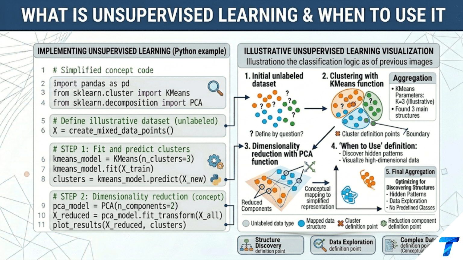
Unsupervised learning finds patterns in data without using labels or predefined correct answers. Instead of learning to predict an output variable, unsupervised algorithms discover the inherent structure of the data itself — grouping similar observations together (clustering), compressing data into fewer dimensions (dimensionality reduction), estimating how data is distributed (density estimation), or identifying unusual observations that don’t fit the learned structure (anomaly detection). The absence of labels makes unsupervised learning harder to evaluate but far more widely applicable, since most real-world data is unlabeled.
Introduction
In supervised learning, every training example comes with a label: this email is spam, that image is a cat, this transaction is fraudulent. The learning algorithm optimizes a model that maps inputs to these known outputs. Supervised learning is powerful, but it has a fundamental constraint — it requires labeled data, which is expensive, slow, and sometimes impossible to obtain.
Most data in the world is unlabeled. Every web page ever written, every sensor reading ever recorded, every image ever uploaded — the overwhelming majority have no attached label telling a learning algorithm what to do with them. Unsupervised learning is how machine learning extracts value from this vast unlabeled majority.
The scope of unsupervised learning is broad. It includes grouping customers by purchasing behavior without knowing what groups exist in advance, compressing 100-dimensional gene expression data to 2 dimensions for visualization, learning that a network request at 3 AM for 50 GB of data is unusual without having a definition of “unusual,” and discovering that news articles cluster into topics without anyone defining what the topics are.
This article provides a thorough introduction to unsupervised learning: its definition, the major problem types it addresses, the key algorithms for each type, how to evaluate methods without labels, and a principled decision framework for choosing the right approach. Every section includes working Python examples.
Supervised vs Unsupervised vs Semi-Supervised Learning
The clearest way to understand unsupervised learning is through contrast with the learning paradigms that bookend it.
import numpy as np
import matplotlib.pyplot as plt
from sklearn.datasets import make_blobs, make_classification
from sklearn.linear_model import LogisticRegression
from sklearn.cluster import KMeans
from sklearn.preprocessing import StandardScaler
import warnings
warnings.filterwarnings('ignore')

np.random.seed(42)


def learning_paradigm_comparison(figsize=(18, 6)):
    """
    Side-by-side visualization of supervised, unsupervised, and
    semi-supervised learning on the same underlying dataset.

    The same two Gaussian blobs are shown three ways:
    - Supervised: boundary learned from labeled data
    - Unsupervised: clusters discovered from unlabeled data
    - Semi-supervised: labels from a few points propagated to all
    """
    X, y_true = make_blobs(n_samples=200, centers=2, cluster_std=0.8,
                            random_state=42)
    scaler = StandardScaler()
    X_s = scaler.fit_transform(X)

    fig, axes = plt.subplots(1, 3, figsize=figsize)
    colors_true = ['coral', 'steelblue']

    # ── Panel 1: Supervised Learning ─────────────────────────────
    ax = axes[0]
    lr = LogisticRegression()
    lr.fit(X_s, y_true)

    x_min, x_max = X_s[:, 0].min() - 0.5, X_s[:, 0].max() + 0.5
    y_min, y_max = X_s[:, 1].min() - 0.5, X_s[:, 1].max() + 0.5
    xx, yy = np.meshgrid(np.linspace(x_min, x_max, 200),
                          np.linspace(y_min, y_max, 200))
    Z = lr.predict(np.c_[xx.ravel(), yy.ravel()]).reshape(xx.shape)

    ax.contourf(xx, yy, Z, alpha=0.2, colors=['#ffd0d0', '#d0e8ff'])
    ax.contour(xx, yy, Z, colors='black', linewidths=1.5, alpha=0.5)
    for cls, color in enumerate(colors_true):
        mask = y_true == cls
        ax.scatter(X_s[mask, 0], X_s[mask, 1], c=color, s=40,
                   edgecolors='white', linewidth=0.5, alpha=0.85,
                   label=f'Class {cls} (labeled)')
    ax.set_title('1. Supervised Learning\n'
                 'Labels provided → learn boundary\n'
                 'Output: decision boundary',
                 fontsize=10, fontweight='bold')
    ax.legend(fontsize=8); ax.grid(True, alpha=0.2)
    ax.set_xlabel('Feature 1', fontsize=9)
    ax.set_ylabel('Feature 2', fontsize=9)

    # ── Panel 2: Unsupervised Learning ───────────────────────────
    ax = axes[1]
    kmeans = KMeans(n_clusters=2, random_state=42, n_init=10)
    cluster_labels = kmeans.fit_predict(X_s)

    cluster_colors = ['mediumpurple', 'goldenrod']
    for clu, color in enumerate(cluster_colors):
        mask = cluster_labels == clu
        ax.scatter(X_s[mask, 0], X_s[mask, 1], c=color, s=40,
                   edgecolors='white', linewidth=0.5, alpha=0.85,
                   label=f'Cluster {clu} (discovered)')
    ax.scatter(kmeans.cluster_centers_[:, 0],
               kmeans.cluster_centers_[:, 1],
               marker='*', s=300, c='black', zorder=5, label='Centroids')
    ax.set_title('2. Unsupervised Learning\n'
                 'No labels → discover structure\n'
                 'Output: cluster assignments',
                 fontsize=10, fontweight='bold')
    ax.legend(fontsize=8); ax.grid(True, alpha=0.2)
    ax.set_xlabel('Feature 1', fontsize=9)

    # ── Panel 3: Semi-Supervised Learning ───────────────────────
    ax = axes[2]
    # Only 10 labeled points; rest are unlabeled
    n_labeled = 10
    labeled_idx = np.random.choice(len(y_true), n_labeled, replace=False)
    y_semi = -np.ones(len(y_true), dtype=int)  # -1 = unlabeled
    y_semi[labeled_idx] = y_true[labeled_idx]

    # Simple label propagation via KNN from labeled → unlabeled
    from sklearn.semi_supervised import LabelPropagation
    lp = LabelPropagation(kernel='knn', n_neighbors=7)
    lp.fit(X_s, y_semi)
    y_propagated = lp.predict(X_s)

    for cls, color in enumerate(colors_true):
        # Unlabeled points that got a propagated label
        mask_unlabeled = (y_semi == -1) & (y_propagated == cls)
        ax.scatter(X_s[mask_unlabeled, 0], X_s[mask_unlabeled, 1],
                   c=color, s=30, edgecolors='white', linewidth=0.3,
                   alpha=0.5, label=f'Class {cls} (propagated)')
        # Labeled points
        mask_labeled = labeled_idx[y_true[labeled_idx] == cls]
        ax.scatter(X_s[mask_labeled, 0], X_s[mask_labeled, 1],
                   c=color, s=150, edgecolors='black', linewidth=2,
                   alpha=1.0, marker='D', zorder=5)

    ax.set_title(f'3. Semi-Supervised Learning\n'
                 f'Only {n_labeled} labels → propagate to all\n'
                 'Output: labels for all points',
                 fontsize=10, fontweight='bold')
    ax.legend(fontsize=7); ax.grid(True, alpha=0.2)
    ax.set_xlabel('Feature 1', fontsize=9)

    plt.suptitle('Three Learning Paradigms on the Same Data\n'
                 '(Diamonds = labeled points in panel 3)',
                 fontsize=13, fontweight='bold', y=1.02)
    plt.tight_layout()
    plt.savefig('learning_paradigms.png', dpi=150, bbox_inches='tight')
    plt.show()
    print("Saved: learning_paradigms.png")


learning_paradigm_comparison()The key distinction is the training signal. Supervised learning has explicit right answers (labels) to learn from. Unsupervised learning has no explicit signal — the algorithm must discover structure that was never defined by anyone. Semi-supervised learning sits in between: a small fraction of data is labeled, and the algorithm uses the unlabeled majority to improve its estimates.
The Four Major Problem Types in Unsupervised Learning
Unsupervised learning is not a single algorithm or technique — it is a collection of problem types, each asking a different question about the structure of data.
1. Clustering: Who Belongs Together?
Clustering partitions data into groups (clusters) such that points within a group are more similar to each other than to points in other groups. No predefined notion of what the groups are or how many there are is required.
Representative algorithms: K-Means, DBSCAN, Hierarchical Clustering, Gaussian Mixture Models, HDBSCAN
Typical use cases:
- Customer segmentation (group customers by behavior without predefined segments)
- Document topic discovery (group articles by theme)
- Image compression (replace each pixel with its cluster’s centroid color)
- Biological taxonomy (group genes or species by expression profiles)
2. Dimensionality Reduction: What Are the Essential Dimensions?
High-dimensional data is difficult to visualize, expensive to store, and problematic for many algorithms (the curse of dimensionality). Dimensionality reduction finds a lower-dimensional representation that preserves the important structure.
Representative algorithms: PCA, t-SNE, UMAP, Autoencoders, ICA
Typical use cases:
- Visualization of high-dimensional data in 2D or 3D
- Feature extraction before supervised learning
- Compression of genomic or image data
- Noise reduction (low-dimensional structure captures signal; discarded dimensions capture noise)
3. Density Estimation: How Is the Data Distributed?
Density estimation models the probability distribution P(x) from which the data was drawn. Rather than assigning points to discrete clusters, it models the continuous distribution.
Representative algorithms: Kernel Density Estimation (KDE), Gaussian Mixture Models (GMM), Normalizing Flows, Variational Autoencoders
Typical use cases:
- Anomaly detection (regions of low probability are anomalous)
- Generative modeling (sample from the learned distribution)
- Bayesian inference (model the prior distribution)
- Hypothesis testing (assess how likely a new observation is)
4. Representation Learning: What Features Should the Model Learn?
Representation learning finds compact, useful internal representations of data. Unlike other unsupervised tasks, the output is an embedding — a new feature vector for each data point that captures semantic structure.
Representative algorithms: Word2Vec, autoencoders, contrastive learning, self-supervised pre-training
Typical use cases:
- Natural language processing (word embeddings that capture semantic similarity)
- Transfer learning (pre-trained representations fine-tuned for downstream tasks)
- Recommendation systems (user and item embeddings)
import numpy as np
import matplotlib.pyplot as plt
from matplotlib.gridspec import GridSpec
from sklearn.datasets import load_digits, make_blobs
from sklearn.cluster import KMeans
from sklearn.decomposition import PCA
from sklearn.neighbors import KernelDensity
from sklearn.preprocessing import StandardScaler


def four_unsupervised_tasks_showcase(figsize=(18, 14)):
    """
    Demonstrate all four unsupervised learning task types on real data.
    """
    # Load digits dataset (1797 images of handwritten digits, 64 features)
    digits = load_digits()
    X_dig, y_dig = digits.data, digits.target
    scaler = StandardScaler()
    X_dig_s = scaler.fit_transform(X_dig)

    fig = plt.figure(figsize=figsize)
    gs  = GridSpec(2, 2, figure=fig, hspace=0.4, wspace=0.35)

    # ── Task 1: Clustering (K-Means on 2D PCA projection) ─────────────
    ax1 = fig.add_subplot(gs[0, 0])
    pca_2d = PCA(n_components=2, random_state=42)
    X_2d = pca_2d.fit_transform(X_dig_s)
    km = KMeans(n_clusters=10, random_state=42, n_init=10)
    clusters = km.fit_predict(X_2d)

    scatter = ax1.scatter(X_2d[:, 0], X_2d[:, 1], c=clusters,
                          cmap='tab10', s=15, alpha=0.7, linewidths=0)
    ax1.scatter(km.cluster_centers_[:, 0], km.cluster_centers_[:, 1],
                marker='*', s=200, c='black', zorder=5)
    ax1.set_title('Task 1: Clustering\nK-Means (k=10) on Digits → Digit-like Groups',
                  fontsize=10, fontweight='bold')
    ax1.set_xlabel('PCA Component 1', fontsize=9)
    ax1.set_ylabel('PCA Component 2', fontsize=9)
    ax1.grid(True, alpha=0.2)

    # ── Task 2: Dimensionality Reduction (PCA variance explained) ──────
    ax2 = fig.add_subplot(gs[0, 1])
    pca_full = PCA(random_state=42)
    pca_full.fit(X_dig_s)
    cumvar = np.cumsum(pca_full.explained_variance_ratio_)
    n_for_95 = np.searchsorted(cumvar, 0.95) + 1

    ax2.plot(range(1, len(cumvar) + 1), cumvar * 100,
             color='steelblue', lw=2.5)
    ax2.axhline(y=95, color='coral', linestyle='--', lw=2,
                label='95% variance threshold')
    ax2.axvline(x=n_for_95, color='coral', linestyle=':', lw=2)
    ax2.fill_between(range(1, n_for_95 + 1),
                     cumvar[:n_for_95] * 100, alpha=0.12, color='steelblue')
    ax2.text(n_for_95 + 2, 50,
             f'{n_for_95} components\nexplain 95%\nof variance',
             fontsize=9, color='coral', fontweight='bold')
    ax2.set_title('Task 2: Dimensionality Reduction\nPCA: 64 → few dimensions',
                  fontsize=10, fontweight='bold')
    ax2.set_xlabel('Number of PCA Components', fontsize=9)
    ax2.set_ylabel('Cumulative Variance Explained (%)', fontsize=9)
    ax2.legend(fontsize=9); ax2.grid(True, alpha=0.3)

    # ── Task 3: Density Estimation (KDE on 2D projection) ─────────────
    ax3 = fig.add_subplot(gs[1, 0])
    # Use just digit 3 and 8 for visual clarity
    mask_38 = np.isin(y_dig, [3, 8])
    X_38 = X_2d[mask_38]
    y_38 = y_dig[mask_38]

    kde = KernelDensity(bandwidth=0.8, kernel='gaussian')
    kde.fit(X_38)

    x_range = np.linspace(X_2d[:, 0].min() - 1, X_2d[:, 0].max() + 1, 100)
    y_range = np.linspace(X_2d[:, 1].min() - 1, X_2d[:, 1].max() + 1, 100)
    XX, YY  = np.meshgrid(x_range, y_range)
    log_dens = kde.score_samples(np.c_[XX.ravel(), YY.ravel()])
    Z_kde   = np.exp(log_dens).reshape(XX.shape)

    ax3.contourf(XX, YY, Z_kde, levels=15, cmap='Blues', alpha=0.7)
    ax3.contour(XX, YY, Z_kde, levels=10, colors='steelblue',
                linewidths=0.8, alpha=0.4)
    for cls, color in [(3, 'coral'), (8, 'goldenrod')]:
        mask = y_38 == cls
        ax3.scatter(X_38[mask, 0], X_38[mask, 1], c=color, s=20,
                    alpha=0.7, label=f'Digit {cls}', edgecolors='white',
                    linewidth=0.3)
    ax3.set_title('Task 3: Density Estimation\nKDE of digit 3 and 8 distributions',
                  fontsize=10, fontweight='bold')
    ax3.set_xlabel('PCA Component 1', fontsize=9)
    ax3.set_ylabel('PCA Component 2', fontsize=9)
    ax3.legend(fontsize=9); ax3.grid(True, alpha=0.2)

    # ── Task 4: Representation Learning (reconstructed images) ─────────
    ax4 = fig.add_subplot(gs[1, 1])
    # Show original vs PCA reconstruction at different n_components
    sample_idx = 7
    x_orig = X_dig[sample_idx]

    n_comp_list = [2, 5, 10, 20, 40, 64]
    recon_errors = []
    for n in n_comp_list:
        pca_n = PCA(n_components=n, random_state=42)
        X_enc = pca_n.fit_transform(X_dig_s)
        X_rec = pca_n.inverse_transform(X_enc)
        X_rec_unscaled = scaler.inverse_transform(X_rec)
        err = np.mean((X_dig - X_rec_unscaled) ** 2)
        recon_errors.append(err)

    ax4.plot(n_comp_list, recon_errors, 'o-', color='mediumseagreen',
             lw=2.5, markersize=8)
    ax4.set_xlabel('Number of PCA Components (latent dim)', fontsize=9)
    ax4.set_ylabel('Mean Reconstruction Error (MSE)', fontsize=9)
    ax4.set_title('Task 4: Representation Learning\n'
                  'PCA reconstruction error vs latent dimension',
                  fontsize=10, fontweight='bold')
    ax4.grid(True, alpha=0.3)

    # Annotate inflection point
    diffs = np.diff(recon_errors)
    inflect_idx = np.argmax(np.abs(diffs) < 1.0) + 1
    if inflect_idx < len(n_comp_list):
        ax4.axvline(x=n_comp_list[inflect_idx], color='coral',
                    linestyle='--', lw=1.5,
                    label=f'Elbow ≈ {n_comp_list[inflect_idx]} dims')
        ax4.legend(fontsize=9)

    plt.suptitle('Four Unsupervised Learning Problem Types\n'
                 'on the Handwritten Digits Dataset',
                 fontsize=14, fontweight='bold', y=1.01)
    plt.savefig('unsupervised_four_tasks.png', dpi=150, bbox_inches='tight')
    plt.show()
    print("Saved: unsupervised_four_tasks.png")


four_unsupervised_tasks_showcase()Evaluating Unsupervised Learning: The Hard Problem
Supervised learning evaluation is straightforward — compare predictions to known labels. Unsupervised learning has no ground truth labels to compare against (by definition), making evaluation fundamentally harder.
Internal Evaluation Metrics (No Labels Needed)
Internal metrics measure the quality of structure discovered using only the data itself.
import numpy as np
from sklearn.datasets import make_blobs, make_moons
from sklearn.cluster import KMeans, DBSCAN
from sklearn.metrics import (silhouette_score, calinski_harabasz_score,
                              davies_bouldin_score)
from sklearn.preprocessing import StandardScaler


def demonstrate_internal_cluster_metrics():
    """
    Three internal clustering quality metrics — all without using labels:

    1. Silhouette Score [-1, 1]: measures cohesion vs separation per point
       Higher = better (well-separated, compact clusters)

    2. Calinski-Harabasz Score [0, ∞): variance ratio criterion
       Higher = better (dense, well-separated clusters)

    3. Davies-Bouldin Score [0, ∞): average similarity ratio
       Lower = better (compact, well-separated clusters)
    """
    np.random.seed(42)

    # Perfect clusters
    X_good, _ = make_blobs(n_samples=300, centers=3, cluster_std=0.4,
                            random_state=42)
    # Overlapping clusters
    X_bad,  _ = make_blobs(n_samples=300, centers=3, cluster_std=2.0,
                            random_state=42)

    datasets = [
        ("Well-separated clusters", X_good),
        ("Overlapping clusters",    X_bad),
        ("Two Moons (true k=2)",    make_moons(300, noise=0.05, random_state=42)[0]),
    ]

    print("=== Internal Clustering Evaluation Metrics ===\n")
    print(f"  {'Dataset':<30} | {'k':>3} | {'Silhouette':>12} | "
          f"{'Calinski-H':>12} | {'Davies-B':>10}")
    print("  " + "-" * 75)

    for ds_name, X in datasets:
        X_s = StandardScaler().fit_transform(X)
        for k in [2, 3, 4]:
            km = KMeans(n_clusters=k, random_state=42, n_init=10)
            labels = km.fit_predict(X_s)

            sil = silhouette_score(X_s, labels)
            ch  = calinski_harabasz_score(X_s, labels)
            db  = davies_bouldin_score(X_s, labels)

            prefix = "→ " if k == 3 and "Well" in ds_name else "  "
            print(f"  {prefix}{ds_name:<28} | {k:>3} | {sil:>12.4f} | "
                  f"{ch:>12.2f} | {db:>10.4f}")
        print()

    print("  Interpretation:")
    print("    Silhouette → highest value = best k")
    print("    Calinski-H → highest value = best k")
    print("    Davies-B   → LOWEST value = best k")
    print("\n  None of these metrics is perfect. Use multiple together.")
    print("  Also plot cluster assignments and visually inspect.")


demonstrate_internal_cluster_metrics()


### External Evaluation Metrics (Ground Truth Available)

def demonstrate_external_cluster_metrics():
    """
    When ground truth labels are available (e.g., in research/testing),
    external metrics compare discovered clusters to true labels.

    ARI (Adjusted Rand Index):     -1 to 1, higher = better match
    NMI (Normalized Mutual Info):   0 to 1, higher = better match
    Homogeneity:                     0 to 1, each cluster = one true class
    Completeness:                    0 to 1, each true class = one cluster
    V-measure:                       harmonic mean of homogeneity + completeness
    """
    from sklearn.metrics import (adjusted_rand_score, normalized_mutual_info_score,
                                  homogeneity_completeness_v_measure)

    np.random.seed(42)
    X, y_true = make_blobs(n_samples=300, centers=3, cluster_std=0.8,
                            random_state=42)
    X_s = StandardScaler().fit_transform(X)

    print("\n=== External Clustering Evaluation (Requires Ground Truth) ===\n")
    print(f"  True k=3, testing k=2,3,4 with K-Means\n")
    print(f"  {'k':>3} | {'ARI':>8} | {'NMI':>8} | {'Homo':>8} | "
          f"{'Comp':>8} | {'V-meas':>8}")
    print("  " + "-" * 55)

    for k in [2, 3, 4]:
        km = KMeans(n_clusters=k, random_state=42, n_init=10)
        pred = km.fit_predict(X_s)

        ari   = adjusted_rand_score(y_true, pred)
        nmi   = normalized_mutual_info_score(y_true, pred)
        h, c, v = homogeneity_completeness_v_measure(y_true, pred)

        best = " ← true k" if k == 3 else ""
        print(f"  {k:>3} | {ari:>8.4f} | {nmi:>8.4f} | {h:>8.4f} | "
              f"{c:>8.4f} | {v:>8.4f}{best}")

    print("\n  ARI=1.0 and NMI=1.0 mean perfect recovery of true clusters.")
    print("  Use external metrics for benchmarking; internal metrics for")
    print("  real applications where ground truth is unavailable.")


demonstrate_external_cluster_metrics()Evaluating Dimensionality Reduction
import numpy as np
from sklearn.decomposition import PCA
from sklearn.datasets import load_digits
from sklearn.preprocessing import StandardScaler
from sklearn.neighbors import KNeighborsClassifier
from sklearn.model_selection import cross_val_score


def evaluate_dimensionality_reduction():
    """
    Three ways to evaluate unsupervised dimensionality reduction:

    1. Reconstruction error: how well can original data be recovered?
    2. Variance explained: how much information is retained?
    3. Downstream task performance: does the low-dim representation help?
    """
    digits = load_digits()
    X, y = digits.data, digits.target
    scaler = StandardScaler()
    X_s = scaler.fit_transform(X)

    n_components_list = [2, 4, 8, 16, 24, 32, 48, 64]

    print("\n=== Dimensionality Reduction Evaluation ===\n")
    print(f"  Digits dataset: {X.shape[1]} features → various reduced dims\n")
    print(f"  {'n_comp':>7} | {'Var Expl%':>10} | {'Recon MSE':>11} | "
          f"{'KNN 5-fold Acc':>15} | Compression")
    print("  " + "-" * 68)

    for n in n_components_list:
        pca = PCA(n_components=n, random_state=42)
        X_reduced = pca.fit_transform(X_s)

        # Variance explained
        var_explained = pca.explained_variance_ratio_.sum() * 100

        # Reconstruction error
        X_recon = pca.inverse_transform(X_reduced)
        X_recon_orig = scaler.inverse_transform(X_recon)
        recon_mse = np.mean((X - X_recon_orig) ** 2)

        # Downstream KNN accuracy
        knn = KNeighborsClassifier(n_neighbors=5)
        knn_acc = cross_val_score(knn, X_reduced, y, cv=5).mean()

        compression = X.shape[1] / n

        print(f"  {n:>7} | {var_explained:>10.2f} | {recon_mse:>11.4f} | "
              f"{knn_acc:>15.4f} | {compression:>5.1f}×")

    print(f"\n  Original 64D KNN accuracy (no reduction):")
    knn_orig = KNeighborsClassifier(n_neighbors=5)
    orig_acc = cross_val_score(knn_orig, X_s, y, cv=5).mean()
    print(f"  {orig_acc:.4f}")
    print(f"\n  A good dimensionality reduction retains downstream accuracy")
    print(f"  while dramatically reducing storage and computation.")


evaluate_dimensionality_reduction()The Curse of Dimensionality: Why Unsupervised Methods Matter
One of the strongest motivations for unsupervised dimensionality reduction is the curse of dimensionality — the phenomenon that high-dimensional spaces behave counterintuitively and make learning harder.
import numpy as np
import matplotlib.pyplot as plt
from scipy.spatial.distance import pdist


def demonstrate_curse_of_dimensionality(n_samples=500, max_dim=1000):
    """
    Three manifestations of the curse of dimensionality:

    1. Distance concentration: in high dimensions, all pairwise distances
       converge to the same value — nearest-neighbor search becomes meaningless.

    2. Volume concentration: almost all volume in a high-dimensional hypersphere
       lies near the surface — the interior is essentially empty.

    3. Data sparsity: the number of samples needed to cover the space
       grows exponentially with dimension.
    """
    np.random.seed(42)
    dims = [1, 2, 5, 10, 20, 50, 100, 200, 500, 1000]

    # 1. Distance concentration
    dist_means = []
    dist_stds  = []
    dist_ratios = []  # (max-min) / mean

    for d in dims:
        X_d = np.random.randn(n_samples, d)
        dists = pdist(X_d[:100], metric='euclidean')  # Pairwise distances
        dist_means.append(dists.mean())
        dist_stds.append(dists.std())
        dist_ratios.append((dists.max() - dists.min()) / dists.mean())

    # 2. Fraction of unit hypercube volume in a thin shell (outer 1%)
    shell_fractions = []
    for d in dims:
        # Volume in outer 1% shell = 1 - 0.99^d
        shell_fractions.append(1 - 0.99 ** d)

    fig, axes = plt.subplots(1, 3, figsize=(16, 5))

    # Panel 1: Relative spread of distances
    ax = axes[0]
    ax.semilogx(dims, dist_ratios, 'o-', color='steelblue', lw=2.5, markersize=8)
    ax.set_xlabel('Dimensionality d', fontsize=11)
    ax.set_ylabel('(max − min dist) / mean dist', fontsize=11)
    ax.set_title('Distance Concentration\n'
                 '(Relative spread → 0: all distances look equal)',
                 fontsize=10, fontweight='bold')
    ax.grid(True, alpha=0.3)
    ax.annotate('Nearest neighbor\nbecomes meaningless\n(all dists ~equal)',
                xy=(dims[-3], dist_ratios[-3]),
                xytext=(dims[-5], dist_ratios[-3] + 0.3),
                fontsize=8, color='coral',
                arrowprops=dict(arrowstyle='->', color='coral'))

    # Panel 2: Volume in thin shell
    ax = axes[1]
    ax.semilogx(dims, np.array(shell_fractions) * 100,
                's-', color='coral', lw=2.5, markersize=8)
    ax.axhline(y=99, color='gray', linestyle='--', lw=1.5, alpha=0.5,
               label='99% of volume in outer shell')
    ax.set_xlabel('Dimensionality d', fontsize=11)
    ax.set_ylabel('% of volume in outer 1% shell', fontsize=11)
    ax.set_title('Volume Concentration\n'
                 'High-d hypercube: almost all volume at boundary',
                 fontsize=10, fontweight='bold')
    ax.legend(fontsize=9); ax.grid(True, alpha=0.3)

    # Panel 3: Samples needed for coverage
    # To cover [0,1]^d with n^d hypercubes needing one sample each: n^d samples
    coverage_dims = [1, 2, 3, 4, 5, 6, 7, 8, 9, 10]
    samples_for_10 = [10 ** d for d in coverage_dims]  # 10 samples per axis

    ax = axes[2]
    ax.semilogy(coverage_dims, samples_for_10, 'o-', color='mediumseagreen',
                lw=2.5, markersize=8)
    ax.axhline(y=1e6, color='coral', linestyle='--', lw=1.5,
               label='1 million samples')
    ax.set_xlabel('Dimensionality d', fontsize=11)
    ax.set_ylabel('Training samples needed (log scale)', fontsize=11)
    ax.set_title('Data Sparsity\n'
                 'Samples needed for coverage grows exponentially',
                 fontsize=10, fontweight='bold')
    ax.legend(fontsize=9); ax.grid(True, alpha=0.3)

    plt.suptitle('The Curse of Dimensionality: Why Dimensionality Reduction Matters',
                 fontsize=13, fontweight='bold')
    plt.tight_layout()
    plt.savefig('curse_of_dimensionality.png', dpi=150)
    plt.show()
    print("Saved: curse_of_dimensionality.png")

    # Summary table
    print(f"\n  {'dim':>6} | {'Dist ratio':>11} | {'Shell %':>9} | Interpretation")
    print("  " + "-" * 55)
    for d, dr, sf in zip(dims[:8], dist_ratios[:8], shell_fractions[:8]):
        interp = ("Distances meaningful" if d <= 5
                  else ("Starting to concentrate" if d <= 20
                        else "All distances ~equal"))
        print(f"  {d:>6} | {dr:>11.4f} | {sf*100:>8.2f}% | {interp}")


demonstrate_curse_of_dimensionality()When to Use Unsupervised Learning: A Decision Framework
The right unsupervised approach depends on the question you are asking, the data you have, and what you will do with the output.
import numpy as np
from sklearn.datasets import load_digits, make_blobs, make_moons
from sklearn.cluster import KMeans, DBSCAN
from sklearn.decomposition import PCA
from sklearn.neighbors import KernelDensity
from sklearn.preprocessing import StandardScaler
from sklearn.ensemble import IsolationForest


def decision_framework_examples():
    """
    Walk through the decision framework with concrete examples.

    Question → Task → Algorithm choice
    """
    np.random.seed(42)
    print("=== Unsupervised Learning Decision Framework ===\n")

    framework = [
        {
            'question':     "Do my customers fall into natural segments?",
            'task':         "Clustering",
            'algorithm':    "K-Means (spherical clusters) or DBSCAN (arbitrary shape)",
            'when_to_use':  "You want to group observations, number of groups unknown",
            'output':       "Cluster assignment per observation",
        },
        {
            'question':     "Can I visualize these 500-dim embeddings?",
            'task':         "Dimensionality Reduction",
            'algorithm':    "t-SNE or UMAP for 2D viz; PCA for preprocessing",
            'when_to_use':  "Too many features; need compression or visualization",
            'output':       "Low-dimensional coordinates per observation",
        },
        {
            'question':     "Which transactions are unusually large/rare?",
            'task':         "Anomaly Detection",
            'algorithm':    "Isolation Forest, One-Class SVM, or LOF",
            'when_to_use':  "Normal behavior is known; anomalies are rare and undefined",
            'output':       "Anomaly score or binary flag per observation",
        },
        {
            'question':     "What topics appear in these 10,000 articles?",
            'task':         "Topic Modeling / Clustering",
            'algorithm':    "LDA (probabilistic) or K-Means on TF-IDF embeddings",
            'when_to_use':  "Discovering latent themes in text without predefined topics",
            'output':       "Topic distribution per document",
        },
        {
            'question':     "How likely is this new data point?",
            'task':         "Density Estimation",
            'algorithm':    "Gaussian Mixture Model or KDE",
            'when_to_use':  "Need probability P(x) for scoring or sampling",
            'output':       "Probability or log-likelihood per observation",
        },
        {
            'question':     "What features should I build for my supervised model?",
            'task':         "Representation / Feature Learning",
            'algorithm':    "PCA (linear) or Autoencoder (nonlinear)",
            'when_to_use':  "Raw features are high-dim, redundant, or noisy",
            'output':       "Dense feature vector per observation",
        },
    ]

    for i, item in enumerate(framework, 1):
        print(f"  {i}. Question: \"{item['question']}\"")
        print(f"     Task:      {item['task']}")
        print(f"     Algorithm: {item['algorithm']}")
        print(f"     Use when:  {item['when_to_use']}")
        print(f"     Output:    {item['output']}")
        print()

    # Quick algorithmic demonstrations of each task type
    print("  Quick demonstrations:\n")

    digits = load_digits()
    X_d, y_d = digits.data, digits.target
    scaler = StandardScaler()
    X_ds = scaler.fit_transform(X_d)

    # Clustering
    pca_2d = PCA(n_components=2, random_state=42)
    X_2d = pca_2d.fit_transform(X_ds)
    km = KMeans(n_clusters=10, random_state=42, n_init=10)
    labels_km = km.fit_predict(X_2d)
    from sklearn.metrics import adjusted_rand_score
    ari = adjusted_rand_score(y_d, labels_km)
    print(f"  Clustering (K-Means, k=10): ARI={ari:.4f} vs true digit labels")

    # Dimensionality reduction
    pca_16 = PCA(n_components=16, random_state=42)
    X_16 = pca_16.fit_transform(X_ds)
    var = pca_16.explained_variance_ratio_.sum()
    print(f"  Dim Reduction (PCA 64→16): {var*100:.1f}% variance retained")

    # Anomaly detection
    iso = IsolationForest(contamination=0.05, random_state=42)
    iso.fit(X_ds)
    scores = iso.score_samples(X_ds)
    n_anomalies = (scores < np.percentile(scores, 5)).sum()
    print(f"  Anomaly Detection (IsoForest): {n_anomalies} flagged anomalies (5%)")

    # Density estimation
    kde = KernelDensity(bandwidth=0.5, kernel='gaussian')
    kde.fit(X_2d)
    log_densities = kde.score_samples(X_2d)
    low_density_count = (log_densities < np.percentile(log_densities, 10)).sum()
    print(f"  Density Estimation (KDE): {low_density_count} low-density points (potential outliers)")


decision_framework_examples()Common Pitfalls in Unsupervised Learning
Understanding when unsupervised methods fail is as important as knowing when they work. The following pitfalls affect nearly every unsupervised project.
import numpy as np
import matplotlib.pyplot as plt
from sklearn.cluster import KMeans
from sklearn.preprocessing import StandardScaler
from sklearn.datasets import make_blobs


def demonstrate_common_pitfalls():
    """
    Four classic unsupervised learning pitfalls with visual demonstrations.
    """
    np.random.seed(42)
    fig, axes = plt.subplots(2, 2, figsize=(14, 12))

    # ── Pitfall 1: Forgetting to scale ────────────────────────────
    ax = axes[0, 0]
    X_raw = np.column_stack([
        np.random.randn(200) * 100,   # Feature 1: range ~[-300, 300]
        np.random.randn(200) * 1,     # Feature 2: range ~[-3, 3]
    ])
    # True clusters: two horizontal bands
    X_raw[100:, 1] += 5

    km_raw = KMeans(n_clusters=2, random_state=42, n_init=10)
    labels_raw = km_raw.fit_predict(X_raw)

    scaler = StandardScaler()
    X_scaled = scaler.fit_transform(X_raw)
    km_scaled = KMeans(n_clusters=2, random_state=42, n_init=10)
    labels_scaled = km_scaled.fit_predict(X_scaled)

    colors = ['coral', 'steelblue']
    for cls, color in enumerate(colors):
        ax.scatter(X_raw[labels_raw == cls, 0],
                   X_raw[labels_raw == cls, 1],
                   c=color, s=20, alpha=0.7, edgecolors='none')

    ax.set_title('Pitfall 1: No Feature Scaling\n'
                 'K-Means dominated by large-scale Feature 1\n'
                 '→ splits vertically, misses horizontal structure',
                 fontsize=9, fontweight='bold')
    ax.set_xlabel('Feature 1 (range ~600)', fontsize=8)
    ax.set_ylabel('Feature 2 (range ~6)', fontsize=8)
    ax.grid(True, alpha=0.2)

    # ── Pitfall 2: Wrong k ─────────────────────────────────────────
    ax = axes[0, 1]
    X_true3, _ = make_blobs(200, centers=3, cluster_std=0.5, random_state=42)

    for wrong_k, marker, label in [(2, 'o', 'k=2 (too few)'),
                                    (6, 's', 'k=6 (too many)')]:
        km_w = KMeans(n_clusters=wrong_k, random_state=42, n_init=10)
        lbl  = km_w.fit_predict(X_true3)
        # Just show centroids, not all points
        ax.scatter(km_w.cluster_centers_[:, 0],
                   km_w.cluster_centers_[:, 1],
                   marker=marker, s=200, label=f'{label}: {wrong_k} centroids',
                   edgecolors='black', linewidth=1.5, zorder=5)

    # Show true k=3
    km_3 = KMeans(n_clusters=3, random_state=42, n_init=10)
    labels_3 = km_3.fit_predict(X_true3)
    for cls in range(3):
        mask = labels_3 == cls
        ax.scatter(X_true3[mask, 0], X_true3[mask, 1],
                   s=15, alpha=0.4, edgecolors='none')
    ax.scatter(km_3.cluster_centers_[:, 0],
               km_3.cluster_centers_[:, 1],
               marker='*', s=300, c='black', zorder=6,
               label='k=3 (correct)')

    ax.set_title('Pitfall 2: Wrong Number of Clusters\n'
                 'Under- and over-clustering both lose information\n'
                 '→ Use elbow method or silhouette score',
                 fontsize=9, fontweight='bold')
    ax.legend(fontsize=7); ax.grid(True, alpha=0.2)

    # ── Pitfall 3: Treating cluster labels as meaningful ───────────
    ax = axes[1, 0]
    np.random.seed(0)
    X_rand = np.random.randn(200, 2)
    km_rand = KMeans(n_clusters=3, random_state=42, n_init=10)
    labels_rand = km_rand.fit_predict(X_rand)

    for cls, color in enumerate(['coral', 'steelblue', 'goldenrod']):
        mask = labels_rand == cls
        ax.scatter(X_rand[mask, 0], X_rand[mask, 1], c=color,
                   s=30, alpha=0.7, edgecolors='white', linewidth=0.3,
                   label=f'Cluster {cls}')
    ax.scatter(km_rand.cluster_centers_[:, 0],
               km_rand.cluster_centers_[:, 1],
               marker='*', s=200, c='black', zorder=5)

    ax.set_title('Pitfall 3: Clustering Random Data\n'
                 'K-Means always finds k clusters — even in noise\n'
                 '→ Always validate: do clusters have real meaning?',
                 fontsize=9, fontweight='bold')
    ax.legend(fontsize=8); ax.grid(True, alpha=0.2)

    # ── Pitfall 4: Using t-SNE distances as a metric ───────────────
    ax = axes[1, 1]
    ax.text(0.5, 0.7,
            "t-SNE Distances Are NOT Meaningful\n\n"
            "• Cluster shapes in t-SNE are arbitrary\n"
            "• Distance between clusters ≠ true distance\n"
            "• Cluster sizes ≠ true sizes\n"
            "• Random seed changes the picture\n\n"
            "t-SNE is for VISUALIZATION ONLY.\n"
            "Never use t-SNE coordinates for:\n"
            "  • Downstream modeling\n"
            "  • Distance-based reasoning\n"
            "  • Quantitative cluster comparison\n\n"
            "Use UMAP or PCA if you need\n"
            "a generalizable embedding.",
            transform=ax.transAxes,
            ha='center', va='center', fontsize=9,
            bbox=dict(boxstyle='round', fc='lightyellow',
                      ec='coral', alpha=0.9))
    ax.set_title('Pitfall 4: Misinterpreting t-SNE\n'
                 'A common visualization mistake',
                 fontsize=9, fontweight='bold')
    ax.axis('off')

    plt.suptitle('Common Unsupervised Learning Pitfalls\n'
                 'Knowing these saves hours of debugging',
                 fontsize=13, fontweight='bold')
    plt.tight_layout()
    plt.savefig('unsupervised_pitfalls.png', dpi=150, bbox_inches='tight')
    plt.show()
    print("Saved: unsupervised_pitfalls.png")


demonstrate_common_pitfalls()Unsupervised Learning in the Machine Learning Pipeline
Unsupervised learning rarely stands alone. In practice it serves as infrastructure that enables or improves supervised learning: dimensionality reduction as preprocessing, clustering as feature engineering, anomaly detection as data cleaning, and representation learning as the backbone of pre-trained models.
| Role in Pipeline | Unsupervised Technique | How It Helps Supervised Learning |
|---|---|---|
| Data cleaning | Anomaly/outlier detection | Remove mislabeled or corrupted samples before training |
| Feature engineering | PCA, autoencoders | Reduce dimensionality, decorrelate features |
| Cluster features | K-Means cluster membership | Add cluster ID as a new feature for downstream models |
| Pre-training | Self-supervised learning | Learn representations from unlabeled data; fine-tune on small labeled set |
| Imbalanced learning | SMOTE (cluster-based oversampling) | Generate synthetic minority-class samples |
| Model debugging | t-SNE / UMAP embedding of predictions | Visualize model errors and confusion regions |
Real-World Case Studies
Understanding how unsupervised learning is applied in practice makes the abstract principles concrete. These five cases each represent a different task type used in production settings.
import numpy as np
import matplotlib.pyplot as plt
from sklearn.datasets import fetch_20newsgroups
from sklearn.feature_extraction.text import TfidfVectorizer
from sklearn.decomposition import TruncatedSVD, PCA
from sklearn.cluster import KMeans
from sklearn.preprocessing import StandardScaler, Normalizer
from sklearn.pipeline import make_pipeline
from sklearn.ensemble import IsolationForest
from sklearn.neighbors import LocalOutlierFactor


def case_study_customer_segmentation():
    """
    Case Study 1: Customer Segmentation
    Simulate an e-commerce customer dataset and discover natural segments.
    """
    np.random.seed(42)
    n_customers = 500

    # Simulated customer features
    # Segment A: High frequency, low spend (budget shoppers)
    # Segment B: Low frequency, high spend (premium buyers)
    # Segment C: Medium frequency, medium spend (regular customers)
    # Segment D: Very low frequency, very low spend (churners)
    segments = {
        'Budget Shoppers':   {'n': 150, 'freq': (20, 3),  'spend': (30, 10)},
        'Premium Buyers':    {'n': 100, 'freq': (4, 1),   'spend': (300, 80)},
        'Regular Customers': {'n': 200, 'freq': (10, 3),  'spend': (100, 25)},
        'Churners':          {'n': 50,  'freq': (1, 0.5), 'spend': (15, 8)},
    }

    rows = []
    true_labels = []
    for i, (name, params) in enumerate(segments.items()):
        n = params['n']
        freq  = np.random.normal(params['freq'][0],  params['freq'][1],  n).clip(0.1)
        spend = np.random.normal(params['spend'][0], params['spend'][1], n).clip(1)
        rows.append(np.column_stack([freq, spend]))
        true_labels.extend([i] * n)

    X_cust = np.vstack(rows)
    true_labels = np.array(true_labels)

    # Scale and cluster
    scaler = StandardScaler()
    X_s = scaler.fit_transform(X_cust)
    km = KMeans(n_clusters=4, random_state=42, n_init=10)
    pred_labels = km.fit_predict(X_s)

    from sklearn.metrics import adjusted_rand_score
    ari = adjusted_rand_score(true_labels, pred_labels)

    print("=== Case Study 1: Customer Segmentation ===\n")
    print(f"  {n_customers} customers, 2 features (purchase frequency, avg spend)\n")
    print(f"  K-Means (k=4) recovered segments with ARI = {ari:.4f}\n")

    # Characterize each cluster
    print("  Discovered Cluster Profiles:\n")
    print(f"  {'Cluster':>8} | {'n':>6} | {'Avg Freq':>10} | {'Avg Spend':>11} | Profile")
    print("  " + "-" * 60)
    for cls in range(4):
        mask = pred_labels == cls
        avg_freq  = X_cust[mask, 0].mean()
        avg_spend = X_cust[mask, 1].mean()
        n_cls     = mask.sum()
        if avg_freq > 12 and avg_spend < 50:
            profile = "Budget Shoppers"
        elif avg_freq < 6 and avg_spend > 200:
            profile = "Premium Buyers"
        elif avg_freq < 3:
            profile = "Churners"
        else:
            profile = "Regular Customers"
        print(f"  {cls:>8} | {n_cls:>6} | {avg_freq:>10.1f} | {avg_spend:>11.1f} | {profile}")


def case_study_text_topic_discovery():
    """
    Case Study 2: Topic Discovery in News Articles
    Use LSA (Latent Semantic Analysis = TF-IDF + SVD) to find topics
    in the 20 Newsgroups dataset without any labels.
    """
    print("\n=== Case Study 2: Text Topic Discovery ===\n")

    # Load 4 categories, strip metadata to avoid leaking labels
    categories = ['sci.space', 'rec.sport.baseball',
                  'comp.graphics', 'talk.politics.guns']
    newsgroups = fetch_20newsgroups(
        subset='train', categories=categories,
        remove=('headers', 'footers', 'quotes'),
        random_state=42
    )
    X_text, y_news = newsgroups.data, newsgroups.target

    # TF-IDF + dimensionality reduction (LSA)
    vectorizer = TfidfVectorizer(max_features=5000, stop_words='english',
                                  min_df=3)
    X_tfidf = vectorizer.fit_transform(X_text)

    svd = TruncatedSVD(n_components=50, random_state=42)
    normalizer = Normalizer(copy=False)
    lsa = make_pipeline(svd, normalizer)
    X_lsa = lsa.fit_transform(X_tfidf)

    # Cluster into topics
    km_text = KMeans(n_clusters=4, random_state=42, n_init=10)
    text_clusters = km_text.fit_predict(X_lsa)

    from sklearn.metrics import adjusted_rand_score, normalized_mutual_info_score
    ari_text = adjusted_rand_score(y_news, text_clusters)
    nmi_text = normalized_mutual_info_score(y_news, text_clusters)

    print(f"  Dataset: {len(X_text)} articles, 4 true topics")
    print(f"  Pipeline: TF-IDF (5000 words) → LSA (50 dims) → K-Means (k=4)\n")
    print(f"  ARI vs true categories: {ari_text:.4f}")
    print(f"  NMI vs true categories: {nmi_text:.4f}\n")

    # Show top words per cluster
    terms = vectorizer.get_feature_names_out()
    original_space_centroids = svd.inverse_transform(km_text.cluster_centers_)
    order_centroids = original_space_centroids.argsort()[:, ::-1]

    cat_map = {i: c.split('.')[-1] for i, c in enumerate(categories)}
    print("  Top words per discovered cluster:")
    for i in range(4):
        top_words = [terms[idx] for idx in order_centroids[i, :8]]
        print(f"  Cluster {i}: {', '.join(top_words)}")


def case_study_anomaly_detection():
    """
    Case Study 3: Network Intrusion / Anomaly Detection
    Simulate normal server requests and a few anomalous ones.
    Compare Isolation Forest and Local Outlier Factor.
    """
    print("\n=== Case Study 3: Anomaly Detection ===\n")
    np.random.seed(42)

    # Normal: requests cluster around typical hours and sizes
    n_normal = 950
    n_anomaly = 50
    normal_hours = np.random.normal(12, 4, n_normal).clip(0, 23)
    normal_size  = np.random.normal(100, 30, n_normal).clip(1)

    # Anomalies: unusual times (late night) and very large sizes
    anom_hours = np.random.uniform(0, 4, n_anomaly)
    anom_size  = np.random.uniform(500, 1000, n_anomaly)

    X_net  = np.column_stack([
        np.concatenate([normal_hours, anom_hours]),
        np.concatenate([normal_size,  anom_size]),
    ])
    y_net  = np.array([0] * n_normal + [1] * n_anomaly)

    scaler = StandardScaler()
    X_net_s = scaler.fit_transform(X_net)

    from sklearn.metrics import roc_auc_score, precision_score, recall_score

    results = {}
    for name, model in [
        ('Isolation Forest', IsolationForest(contamination=0.05, random_state=42)),
        ('LOF',              LocalOutlierFactor(contamination=0.05, novelty=False)),
    ]:
        if name == 'LOF':
            scores = -model.fit_predict(X_net_s)  # -1=anomaly, 1=normal
            preds  = (scores > 0).astype(int)
            auc    = roc_auc_score(y_net, -model.negative_outlier_factor_)
        else:
            model.fit(X_net_s)
            preds  = (model.predict(X_net_s) == -1).astype(int)
            auc    = roc_auc_score(y_net, -model.score_samples(X_net_s))

        prec   = precision_score(y_net, preds)
        rec    = recall_score(y_net, preds)
        results[name] = (auc, prec, rec)

    print(f"  {n_normal} normal requests + {n_anomaly} anomalies (late-night, large)\n")
    print(f"  {'Model':<20} | {'AUC-ROC':>9} | {'Precision':>10} | {'Recall':>8}")
    print("  " + "-" * 52)
    for name, (auc, prec, rec) in results.items():
        print(f"  {name:<20} | {auc:>9.4f} | {prec:>10.4f} | {rec:>8.4f}")

    print("\n  Key insight: Anomaly detection requires NO labeled examples of")
    print("  anomalies — the model learns normal behavior and flags deviations.")


# Run all case studies
case_study_customer_segmentation()
case_study_text_topic_discovery()
case_study_anomaly_detection()These three case studies illustrate the breadth of unsupervised learning in practice. Customer segmentation discovers actionable groups that inform marketing strategy without requiring anyone to predefine what a segment is. Text topic discovery distills thousands of articles into interpretable themes using only word co-occurrence patterns. Anomaly detection identifies security threats without ever having seen a labeled attack — it learns what normal looks like and flags deviations.
Each case study also illustrates a fundamental characteristic of unsupervised learning: the results require domain expert interpretation. K-Means returns cluster 0, 1, 2, 3 — a human labels them “Budget Shoppers” and “Premium Buyers.” LSA returns mathematical topics — a human reads the top words and assigns the label “Space” or “Baseball.” The algorithm discovers structure; the domain expert interprets it.
Summary
Unsupervised learning addresses the most fundamental form of pattern recognition: finding structure in data without being told what structure to look for. Its four major problem types — clustering, dimensionality reduction, density estimation, and representation learning — each address a different question about the data’s hidden organization.
The absence of labels makes unsupervised evaluation fundamentally harder than supervised evaluation. Internal metrics (silhouette score, Davies-Bouldin index) measure the quality of discovered structure without reference to ground truth. External metrics (ARI, NMI) quantify how well discovered structure aligns with known labels when available. Downstream task performance — how much a supervised model improves after unsupervised preprocessing — provides the most practically meaningful evaluation.
The curse of dimensionality is a primary motivation for unsupervised dimensionality reduction: in high-dimensional spaces, distances concentrate, volumes empty, and the amount of data needed for coverage grows exponentially. Unsupervised methods that discover the low-dimensional manifold embedded in high-dimensional data are therefore not just convenient but often necessary.
Coming articles will cover the major algorithms in each unsupervised category: K-Means and DBSCAN for clustering, PCA and t-SNE for dimensionality reduction, and Gaussian Mixture Models for density estimation. Each algorithm embodies a different assumption about the structure of data, and understanding those assumptions is the key to knowing when each technique will succeed or fail.