A data warehouse is a centralized analytical database that consolidates data from multiple operational systems — sales platforms, CRM systems, product databases, financial tools — into a single, integrated store optimized for reporting and analysis rather than transaction processing. Data warehouses organize data into fact tables (which record events and measurements like sales transactions) and dimension tables (which provide context like customer, product, and date information), connected in a star schema pattern. Modern cloud data warehouses like BigQuery, Snowflake, and Redshift can store petabytes of data and execute analytical queries across billions of rows in seconds, making them the primary data source for data scientists in enterprise environments.
Introduction
Walk into any large technology company, financial institution, retailer, or healthcare organization and ask where their analytical data lives. The answer, almost universally, involves a data warehouse. It might be called different things — the analytics layer, the reporting database, the data platform, the gold layer — but the underlying concept is the same: a centralized repository where cleaned, integrated, historical data lives and where analysts, data scientists, and business intelligence tools come to ask questions.
For data scientists, understanding data warehousing concepts is not optional background knowledge — it is a prerequisite for effective work in almost any organizational setting. You need to know why the data is structured the way it is, what a fact table versus a dimension table is, why your query is joining to a “dim_” prefixed table, what the “SCD” columns mean, why some historical records have date ranges instead of single dates, and why aggregating across certain combinations of dimensions produces unexpected results.
This article provides the conceptual foundation: what data warehouses are and why they exist, the architectural patterns that organize warehouse data (star schema, snowflake schema), the building blocks of dimensional modeling (facts, dimensions, slowly changing dimensions), the modern evolution toward data lakes and lakehouses, and the practical skills for working effectively with warehouse data as a data scientist.
The Problem Data Warehouses Solve
To understand data warehouses, start with the problem they solve.
Operational Systems Are Not Designed for Analysis
Every organization runs operational systems — also called OLTP systems (Online Transaction Processing) — that handle day-to-day business activities:
- An e-commerce platform records purchases, updates inventory, and processes payments
- A CRM system tracks customer interactions and support tickets
- A finance system processes invoices and payroll
- A product database manages catalog information and pricing
These systems are optimized for a specific workload: many small, fast read-write transactions. When a customer places an order, the system must look up their address, check inventory, decrement stock, record the transaction, and send a confirmation — all in milliseconds.
OLTP databases are designed for this: normalized schemas (data split into many small tables to minimize redundancy), row-oriented storage (optimized for reading and writing complete records one at a time), and indices on primary keys for fast single-row lookups.
This design is terrible for analytical queries. Consider: “What was the month-over-month revenue growth by product category for each geographic region over the past three years, and how does it correlate with our marketing spend?” This query needs to:
- Scan millions of transaction records
- Join across orders, products, customers, and marketing tables
- Aggregate across time, geography, and category dimensions
- Compare across multiple time periods
Running this against a production OLTP database would lock tables, slow down real customers, and probably time out anyway. The query patterns are fundamentally different.
The OLTP vs. OLAP Distinction
| Characteristic | OLTP | OLAP (Data Warehouse) |
|---|---|---|
| Primary purpose | Run the business | Analyze the business |
| Query pattern | Many small reads/writes | Few large reads, no writes |
| Data volume | Current state | Historical accumulation |
| Schema design | Normalized (many small tables) | Denormalized (fewer wide tables) |
| Optimization | Fast single-row operations | Fast multi-row aggregations |
| Users | Applications, software | Analysts, data scientists, BI tools |
| Update frequency | Constant (every transaction) | Batch (nightly or hourly) |
| Time horizon | Now (current state) | History (trends over time) |
| Example systems | PostgreSQL, MySQL, Oracle | BigQuery, Snowflake, Redshift |
OLAP stands for Online Analytical Processing — queries that scan large volumes of data to compute aggregations, identify trends, and answer business questions.
Data warehouses are OLAP systems: they store historical data, are designed for complex analytical queries, and are separated from production OLTP systems to prevent analytical workloads from impacting operational performance.
The Architecture of a Data Warehouse
Data warehouses don’t just receive raw operational data — they transform and organize it. The classic architecture flows through several layers:
The Three-Layer Architecture
Source Systems                          Landing / Staging
(OLTP databases,            ──ETL──►    (Raw data, as-is from
 APIs, flat files,                       source systems, minimal
 event streams)                          transformation)
                                                    │
                                                    ▼
                                        Core / Integration
                                        (Cleansed, standardized,
                                         integrated data; business
                                         key mapping)
                                                    │
                                                    ▼
                                        Presentation / Data Mart
                                        (Star schemas, subject-area
                                         marts for analysts and BI)
                                                    │
                                                    ▼
                                        Analysts / Data Scientists
BI Tools / Dashboards / ML ModelsStaging layer: Raw data from source systems, loaded as-is with minimal transformation. Serves as an audit trail — you can always trace back to what was received from the source.
Core layer (also called the integration layer or ODS — Operational Data Store): Cleaned, standardized data. Business keys mapped to warehouse surrogate keys. Data quality rules applied. All sources integrated into a consistent model.
Presentation layer (also called the data mart layer): Dimensional models (star schemas) organized by subject area — a sales mart, a customer mart, a finance mart. Optimized for query performance and ease of use by analysts.
Modern cloud warehouses and dbt-based pipelines often use a similar three-layer pattern called bronze (raw) → silver (cleaned) → gold (aggregated/marts), which we’ll revisit in the data lakehouse section.
Dimensional Modeling: The Language of Data Warehouses
Dimensional modeling is the methodology for organizing data warehouse tables. Developed by Ralph Kimball and published in “The Data Warehouse Toolkit” (1996), it remains the dominant framework for analytical data modeling today.
The core insight: separate the measurements of business events (what happened, how much, how many) from the context of those events (who, what, where, when, why).
Measurements live in fact tables. Context lives in dimension tables.
Fact Tables: What Happened
A fact table records business events or measurements. Each row represents a specific event at the declared grain of the table.
import pandas as pd

# Sales fact table (order-item grain — one row per line item per order)
sales_fact = pd.DataFrame({
    # Surrogate foreign keys — these are integers that join to dimension tables
    "order_item_key":  [1, 2, 3, 4, 5],
    "order_date_key":  [20240901, 20240901, 20240903, 20240905, 20240905],
    "customer_key":    [1001, 1001, 1002, 1003, 1003],
    "product_key":     [501, 502, 501, 503, 504],
    "store_key":       [201, 201, 201, 202, 202],
    "promotion_key":   [0, 0, 301, 0, 301],  # 0 = no promotion

    # Measures — the numeric "facts" being recorded
    "quantity_sold":   [2, 1, 3, 1, 2],
    "unit_price":      [149.99, 49.99, 149.99, 89.99, 29.99],
    "discount_amount": [0.00, 0.00, 15.00, 4.50, 0.00],
    "line_revenue":    [299.98, 49.99, 434.97, 85.49, 59.98],
    "cost_of_goods":   [90.00, 20.00, 90.00, 45.00, 12.00],
    "gross_profit":    [209.98, 29.99, 344.97, 40.49, 47.98]
})

print("Sales fact table:")
print(sales_fact)
print(f"\nGrain: one row per order line item (order_item_key is unique)")Key properties of fact tables:
- Rows represent events at a specific grain (defined by the combination of dimension keys)
- Contain mostly foreign keys (linking to dimensions) and measures (numeric facts)
- Can be very large — billions of rows for high-volume business processes
- Typically narrow in the dimension key columns, with many measure columns
- Additive measures (revenue, quantity) can be summed across all dimensions; semi-additive measures (inventory balance) only across some; non-additive measures (unit price, ratios) cannot be summed
Types of fact tables:
Transaction fact (finest grain): One row per event
├── Sales order line items
├── Web clickstream events
└── Financial transactions

Periodic snapshot: One row per entity per period
├── Account balances (one row per account per month)
├── Inventory levels (one row per product per day)
└── Customer health scores (one row per customer per week)

Accumulating snapshot: One row per process instance, updated as it progresses
├── Order fulfillment (one row per order, updated from placed → shipped → delivered)
├── Loan origination (one row per application, updated through stages)
└── Customer onboarding (one row per customer, tracks completion of steps)Dimension Tables: The Context
Dimension tables provide the descriptive context that makes measurements meaningful. They answer the who, what, where, and when of each fact.
# Customer dimension table
customer_dim = pd.DataFrame({
    # Surrogate key (warehouse-generated, never changes)
    "customer_key": [1001, 1002, 1003, 1004],

    # Natural/business key (from the source system)
    "customer_id":  ["CUST_001", "CUST_002", "CUST_003", "CUST_004"],

    # Descriptive attributes — lots of them
    "first_name":   ["Jane",   "Bob",   "Alice",  "Carlos"],
    "last_name":    ["Smith",  "Johnson","Williams","Garcia"],
    "email":        ["jane@email.com", "bob@email.com",
                     "alice@email.com", "carlos@email.com"],
    "city":         ["Austin", "Seattle", "Chicago", "Miami"],
    "state":        ["TX",     "WA",      "IL",      "FL"],
    "country":      ["USA",    "USA",     "USA",     "USA"],
    "region":       ["South",  "West",    "Midwest", "South"],
    "age_band":     ["35-44",  "25-34",   "45-54",   "25-34"],
    "income_band":  ["75-100K","50-75K",  "100K+",   "50-75K"],
    "customer_segment": ["Premium", "Standard", "Premium", "Standard"],
    "acquisition_channel": ["Organic", "Paid Search", "Referral", "Email"],

    # Record metadata (for slowly changing dimensions — discussed later)
    "effective_date": pd.to_datetime(["2022-03-14", "2021-11-28",
                                       "2023-01-05", "2022-07-19"]),
    "expiry_date":    pd.to_datetime(["9999-12-31", "9999-12-31",
                                       "9999-12-31", "9999-12-31"]),
    "is_current":     [True, True, True, True]
})

# Date dimension table — one row per calendar date, pre-populated years in advance
date_dim = pd.DataFrame({
    "date_key":    [20240901, 20240902, 20240903, 20240904, 20240905],
    "full_date":   pd.to_datetime(["2024-09-01", "2024-09-02", "2024-09-03",
                                    "2024-09-04", "2024-09-05"]),
    "day_of_week": ["Sunday", "Monday", "Tuesday", "Wednesday", "Thursday"],
    "is_weekend":  [True, False, False, False, False],
    "week_number": [35, 36, 36, 36, 36],
    "month_number":[9, 9, 9, 9, 9],
    "month_name":  ["September"] * 5,
    "quarter":     [3, 3, 3, 3, 3],
    "year":        [2024] * 5,
    "is_holiday":  [False, False, False, False, False],
    "fiscal_year": [2025] * 5,    # Company fiscal year may differ from calendar
    "fiscal_quarter": ["FQ1"] * 5
})

# Product dimension table
product_dim = pd.DataFrame({
    "product_key":      [501, 502, 503, 504],
    "product_id":       ["PROD_001", "PROD_002", "PROD_003", "PROD_004"],
    "product_name":     ["Wireless Headphones", "USB-C Hub", "Running Shoes", "Yoga Mat"],
    "brand":            ["SoundMax", "TechGear", "FitStride", "ZenFlex"],
    "subcategory":      ["Audio", "Accessories", "Athletic Footwear", "Fitness Equipment"],
    "category":         ["Electronics", "Electronics", "Apparel", "Sports"],
    "department":       ["Technology", "Technology", "Fashion", "Health"],
    "unit_cost":        [45.00, 20.00, 45.00, 12.00],
    "list_price":       [149.99, 49.99, 89.99, 29.99],
    "is_active":        [True, True, True, True]
})

print("Product dimension table:")
print(product_dim[["product_key", "product_name", "category", "list_price"]])Key properties of dimension tables:
- Relatively small compared to fact tables (thousands to millions of rows, not billions)
- Wide — many descriptive columns (50-100+ columns is common in large dimensions)
- Contain the surrogate key (warehouse-generated) and the natural/business key (from the source)
- Include all the attributes users want to group by, filter on, or display in reports
- The date dimension is special — pre-populated with every calendar date for decades, with all possible temporal attributes pre-computed
The Star Schema
The star schema is the most common dimensional model pattern. It gets its name from its visual structure: a fact table at the center with dimension tables radiating outward like the points of a star.
[date_dim]
                            |
                            | date_key
                            |
[store_dim] ──store_key── [sales_fact] ──product_key── [product_dim]
                            |
                            | customer_key
                            |
                        [customer_dim]
                            |
                            | promotion_key
                            |
[promotion_dim]import pandas as pd
# Star schema query: revenue by category and region for Q3 2024
def star_schema_query(sales_fact, date_dim, customer_dim, product_dim):
"""
Demonstrate a star schema join — the fundamental analytical query pattern.
"""
# Step 1: Join fact to date dimension to filter to Q3 2024
with_date = sales_fact.merge(
date_dim[["date_key", "quarter", "year", "month_name"]],
on="date_key",
how="inner"
)
q3_2024 = with_date[(with_date["year"] == 2024) &
(with_date["quarter"] == 3)]
# Step 2: Join to customer dimension for geographic context
with_customer = q3_2024.merge(
customer_dim[["customer_key", "region", "customer_segment"]],
on="customer_key",
how="inner"
)
# Step 3: Join to product dimension for category context
with_product = with_customer.merge(
product_dim[["product_key", "category", "department"]],
on="product_key",
how="inner"
)
# Step 4: Aggregate — this is what the analyst actually wants
result = (
with_product
.groupby(["region", "category"])
.agg(
total_revenue = ("line_revenue", "sum"),
total_units = ("quantity_sold", "sum"),
gross_profit = ("gross_profit", "sum"),
n_transactions = ("order_item_key", "count")
)
.reset_index()
.sort_values("total_revenue", ascending=False)
)
result["margin_pct"] = (result["gross_profit"] / result["total_revenue"] * 100).round(1)
return result
revenue_by_region_category = star_schema_query(
sales_fact, date_dim, customer_dim, product_dim
)
print(revenue_by_region_category)Why the Star Schema Works for Analysis
The star schema trades storage efficiency (denormalization means some redundancy) for query simplicity and performance:
Simple queries: Every analytical question follows the same pattern — start at the fact table, join to the relevant dimensions, filter and aggregate. Analysts learn one pattern that works everywhere.
Fast queries: Modern columnar warehouses execute star schema joins extremely efficiently. The fact table is columnar (fast scans), dimension tables fit in memory or are cached (fast lookups), and the query optimizer knows how to handle this well-understood pattern.
Self-documenting: The naming conventions (dim_customer, fact_sales) make the model’s intent obvious. Foreign keys in the fact table clearly point to their dimension tables.
The Snowflake Schema
A snowflake schema normalizes the dimension tables further — subcategory is a separate table joined to category, city is a separate table joined to state, which is joined to country. This reduces storage redundancy but requires more joins in queries and is generally harder to use.
                   [dim_product]
                         |
                product_category_key
                         |
               [dim_product_category]
                         |
                   department_key
                         |
[dim_department]Most practitioners prefer star schemas (denormalized dimensions) over snowflake schemas because:
- Storage is cheap; query complexity is expensive
- Fewer joins mean simpler queries and better performance
- Dimension tables are small — the redundancy cost is minimal
Surrogate Keys vs. Natural Keys
One of the most important (and initially confusing) design patterns in dimensional modeling is the use of surrogate keys.
Natural key: The business identifier from the source system. customer_id = "CUST_001", product_sku = "HDPH-PRO-WH". These are meaningful but can change, can be recycled, and may not be unique across multiple source systems.
Surrogate key: A warehouse-generated integer that uniquely identifies each dimension record. customer_key = 1001. Has no business meaning — just a join key.
import pandas as pd

# Why surrogate keys matter: the same natural key can mean different things over time

# Original customer record
customer_v1 = {
    "customer_key": 1001,         # Surrogate: never changes
    "customer_id":  "CUST_001",   # Natural key: stays the same
    "name":         "Jane Smith",
    "city":         "Austin",
    "segment":      "Standard",
    "effective_date": "2022-03-14",
    "expiry_date":    "2024-06-30",
    "is_current":     False
}

# Customer moved and was promoted — NEW surrogate key for the new version
customer_v2 = {
    "customer_key": 5823,         # New surrogate key for new record
    "customer_id":  "CUST_001",   # Same natural key (same person)
    "name":         "Jane Smith-Torres",
    "city":         "San Francisco",
    "segment":      "Premium",
    "effective_date": "2024-07-01",
    "expiry_date":    "9999-12-31",
    "is_current":     True
}

# Historical sales facts JOIN to customer_key=1001 → "Jane was Standard in Austin"
# Recent sales facts JOIN to customer_key=5823 → "Jane is Premium in San Francisco"
# Natural key alone can't distinguish these two statesSlowly Changing Dimensions (SCD)
Dimension attributes change over time — customers move, products are recategorized, employees change departments. Slowly Changing Dimensions (SCDs) define how to handle these changes in a warehouse.
SCD Type 1: Overwrite (No History)
The simplest approach: just update the record. No history is preserved.
# SCD Type 1: Update in place — lose the history
# BEFORE: Jane lives in Austin, segment=Standard
customer_dim.loc[customer_dim["customer_key"] == 1001, "city"] = "San Francisco"
customer_dim.loc[customer_dim["customer_key"] == 1001, "segment"] = "Premium"
# AFTER: Jane now shows San Francisco/Premium for ALL historical facts too
# Historical analysis is permanently affected — intended for corrections, not real changesUse SCD Type 1 when: the change is a correction (a typo was fixed), when history genuinely doesn’t matter (a field being added retroactively), or when storage is very limited.
SCD Type 2: Add New Row (Full History)
The most commonly used SCD type: add a new row for each change, preserving the old row with its effective date range.
import pandas as pd

def scd_type_2_update(
    dim_df: pd.DataFrame,
    natural_key_col: str,
    natural_key_value: str,
    updates: dict,
    change_date: str,
    surrogate_key_col: str = "surrogate_key"
) -> pd.DataFrame:
    """
    Apply a SCD Type 2 update to a dimension table.

    Expires the current record (sets expiry_date and is_current=False)
    and inserts a new record with the updated attribute values.

    Parameters
    ----------
    dim_df : pd.DataFrame
        The dimension table to update.
    natural_key_col : str
        Column containing the business/natural key.
    natural_key_value : str
        Value of the natural key for the record being updated.
    updates : dict
        Dict of {column_name: new_value} for changed attributes.
    change_date : str
        Date the change became effective (ISO format string).
    surrogate_key_col : str
        Name of the surrogate key column.

    Returns
    -------
    pd.DataFrame
        Updated dimension table with expired old record and new current record.
    """
    dim_df = dim_df.copy()
    change_ts = pd.Timestamp(change_date)

    # Find the current active record
    current_mask = (
        (dim_df[natural_key_col] == natural_key_value) &
        (dim_df["is_current"] == True)
    )
    current_record = dim_df[current_mask].iloc[0].to_dict()

    # Expire the current record
    dim_df.loc[current_mask, "expiry_date"] = change_ts - pd.Timedelta(days=1)
    dim_df.loc[current_mask, "is_current"]  = False

    # Create the new record
    new_record = current_record.copy()
    new_record.update(updates)
    new_record["effective_date"] = change_ts
    new_record["expiry_date"]    = pd.Timestamp("9999-12-31")
    new_record["is_current"]     = True
    # Generate new surrogate key
    new_record[surrogate_key_col] = dim_df[surrogate_key_col].max() + 1

    # Append new record
    new_row_df = pd.DataFrame([new_record])
    dim_df = pd.concat([dim_df, new_row_df], ignore_index=True)

    return dim_df


# Apply SCD Type 2: Jane moved to San Francisco and was upgraded to Premium
customer_dim_updated = scd_type_2_update(
    customer_dim,
    natural_key_col="customer_id",
    natural_key_value="CUST_001",
    updates={"city": "San Francisco", "state": "CA",
              "region": "West", "customer_segment": "Premium"},
    change_date="2024-07-01",
    surrogate_key_col="customer_key"
)

jane_records = customer_dim_updated[
    customer_dim_updated["customer_id"] == "CUST_001"
][["customer_key", "city", "customer_segment", "effective_date", "expiry_date", "is_current"]]

print("Jane Smith's dimension history after SCD Type 2 update:")
print(jane_records.to_string(index=False))Output:
customer_key     city  customer_segment effective_date  expiry_date  is_current
        1001   Austin          Standard     2022-03-14   2024-06-30       False
1005 San Francisco Premium 2024-07-01 9999-12-31 TrueNow historical sales facts that join to customer_key=1001 correctly show Jane as “Standard/Austin” for her old purchases, while recent sales join to customer_key=1005 and show “Premium/San Francisco.”
SCD Type 3: Add New Column (Limited History)
Adds a new column to preserve the previous value — only one level of history:
# SCD Type 3: Keep both current and previous values
customer_dim_type3 = pd.DataFrame({
    "customer_key":         [1001],
    "customer_id":          ["CUST_001"],
    "name":                 ["Jane Smith"],
    # Current values
    "current_city":         ["San Francisco"],
    "current_segment":      ["Premium"],
    # Previous values (one level of history only)
    "previous_city":        ["Austin"],
    "previous_segment":     ["Standard"],
    # When the change happened
    "last_change_date":     pd.to_datetime(["2024-07-01"])
})SCD Type 3 is simple but limited — it only stores the most recent previous value. If Jane moved three times, only the last previous city is preserved. Use it when you only need to compare current vs. previous and space is very constrained.
Date Dimension: The Special Case
The date dimension is the most universally present dimension in any warehouse. Unlike other dimensions, it’s static — every possible date is pre-populated at warehouse setup time.
import pandas as pd
import numpy as np

def build_date_dimension(start_date: str = "2020-01-01",
                          end_date: str   = "2030-12-31") -> pd.DataFrame:
    """
    Build a comprehensive date dimension table.

    Pre-computes every possible temporal attribute for every date
    so that queries can filter and group without date functions.

    Parameters
    ----------
    start_date, end_date : str
        Date range for the dimension (cover all historical + future dates).

    Returns
    -------
    pd.DataFrame
        One row per calendar date with all temporal attributes.
    """
    dates = pd.date_range(start=start_date, end=end_date, freq="D")

    df = pd.DataFrame({
        # Surrogate key as integer YYYYMMDD — easy to remember and use
        "date_key":         dates.strftime("%Y%m%d").astype(int),
        "full_date":        dates,

        # Calendar attributes
        "year":             dates.year,
        "quarter":          dates.quarter,
        "month_number":     dates.month,
        "month_name":       dates.strftime("%B"),
        "month_abbrev":     dates.strftime("%b"),
        "week_of_year":     dates.isocalendar().week.astype(int),
        "day_of_year":      dates.day_of_year,
        "day_of_month":     dates.day,
        "day_of_week":      dates.dayofweek,     # 0=Mon
        "day_name":         dates.strftime("%A"),
        "day_abbrev":       dates.strftime("%a"),

        # Boolean flags
        "is_weekday":       dates.dayofweek < 5,
        "is_weekend":       dates.dayofweek >= 5,
        "is_month_start":   dates.is_month_start,
        "is_month_end":     dates.is_month_end,
        "is_quarter_start": dates.is_quarter_start,
        "is_quarter_end":   dates.is_quarter_end,
        "is_year_start":    dates.is_year_start,
        "is_year_end":      dates.is_year_end,

        # Formatted strings for display
        "year_month":       dates.strftime("%Y-%m"),
        "year_quarter":     dates.strftime("%Y") + "-Q" + dates.quarter.astype(str),
        "month_year_label": dates.strftime("%b %Y"),

        # Fiscal year (example: fiscal year starts October 1)
        "fiscal_year":      np.where(dates.month >= 10,
                                      dates.year + 1, dates.year),
        "fiscal_quarter":   np.select(
            [dates.month.isin([10,11,12]), dates.month.isin([1,2,3]),
             dates.month.isin([4,5,6])],
            [1, 2, 3], default=4
        )
    })

    return df

date_dim_full = build_date_dimension("2020-01-01", "2030-12-31")
print(f"Date dimension: {len(date_dim_full):,} rows")
print(date_dim_full.loc[date_dim_full["full_date"] == "2024-09-15"].T)The date dimension is used in every analytical query involving time. Pre-computing is_weekend, fiscal_quarter, month_name, and hundreds of other attributes eliminates the need for date functions in analytical queries — queries join to the date dimension and filter like WHERE is_weekend = TRUE rather than computing day-of-week at query time.
Data Lakes and Lakehouses
While the traditional data warehouse model has served organizations well, the past decade has seen significant architectural evolution driven by the rise of big data and cloud storage.
The Traditional Warehouse Limitations
Traditional data warehouses had real constraints:
- Schema-on-write: Data must conform to a defined schema before loading. Unstructured or semi-structured data (text, images, logs) couldn’t be stored.
- Expensive scaling: Adding storage and compute meant adding hardware — expensive and slow.
- One team controls it: Centralized governance meant data teams controlled what could be analyzed and by whom.
- Not for ML: Training machine learning models on raw logs or unstructured data required exporting to a separate system.
The Data Lake
A data lake stores raw data of any type — structured, semi-structured (JSON, XML), unstructured (text, images, audio) — in cheap cloud object storage (Amazon S3, Google Cloud Storage, Azure Blob Storage) in whatever format it arrives.
The core idea: schema-on-read — define the schema when you query the data, not when you store it. This gives maximum flexibility: store everything now, figure out how to use it later.
Data Lake (e.g., Amazon S3)
├── raw/
│   ├── transactions/year=2024/month=09/day=15/txns_001.parquet
│   ├── clickstream/2024-09-15/events_000.jsonl
│   ├── customer_uploads/profile_photos/
│   └── third_party/weather_data/station_readings_2024.csv
├── processed/
│   ├── transactions_cleaned/
│   └── customer_features/
└── ml_datasets/
    ├── churn_training_v3/
    └── recommendation_training/
Data lakes are cheap and flexible, but they create problems: data quality is inconsistent, there’s no governance about what’s in there, data scientists might work from stale or corrupted data, and query performance can be poor on raw JSON/CSV.
The Data Lakehouse
The data lakehouse architecture (popularized by Databricks and reflected in Delta Lake, Apache Iceberg, and Apache Hudi) combines the flexibility of a data lake with the reliability and performance of a data warehouse.
The key innovation is a transactional metadata layer on top of object storage that provides:
- ACID transactions: Consistent reads and writes, even with concurrent users
- Schema enforcement: Optional: define a schema and reject data that doesn’t conform
- Time travel: Query historical versions of the data
- Streaming + batch: Handle both real-time events and batch loads in the same table
# Delta Lake example (Apache Spark + Delta)
from delta.tables import DeltaTable
from pyspark.sql import SparkSession

spark = SparkSession.builder \
    .config("spark.sql.extensions", "io.delta.sql.DeltaSparkSessionExtension") \
    .getOrCreate()

# Write a Delta table
df.write.format("delta").save("s3://bucket/delta/transactions/")

# ACID merge (upsert) — not possible with plain Parquet
delta_table = DeltaTable.forPath(spark, "s3://bucket/delta/transactions/")
delta_table.alias("existing").merge(
    new_data.alias("updates"),
    "existing.transaction_id = updates.transaction_id"
).whenMatchedUpdateAll() \
 .whenNotMatchedInsertAll() \
 .execute()

# Time travel: query yesterday's version
df_yesterday = spark.read.format("delta") \
    .option("timestampAsOf", "2024-09-14") \
    .load("s3://bucket/delta/transactions/")

# Query a specific version
df_v5 = spark.read.format("delta") \
    .option("versionAsOf", 5) \
.load("s3://bucket/delta/transactions/")The Modern Data Stack
Today’s data infrastructure often combines:
Source Systems (OLTP)
        │
        ▼
Ingestion (Fivetran, Airbyte, Kafka)
        │
        ▼
Cloud Object Storage (S3, GCS) — the data lake
        │
        ▼
Cloud Data Warehouse (Snowflake, BigQuery, Redshift)
  OR Data Lakehouse (Databricks, Delta Lake, Apache Iceberg)
        │
        ▼
Transformation (dbt — SQL-based transformation tool)
        │
        ▼
Presentation Layer (dimensional models, marts)
        │
        ├──► BI Tools (Tableau, Looker, Power BI)
        ├──► Analytics (SQL + Python notebooks)
└──► ML (Feature stores, model training)dbt (data build tool) deserves special mention: it is the most widely adopted transformation tool in the modern data stack, allowing data teams to write SQL SELECT statements that define data models, with version control, testing, documentation, and dependency management built in.
Working with Warehouse Data as a Data Scientist
Understanding warehouse architecture makes you more effective at extracting data for analysis and modeling.
Navigating a New Warehouse
import pandas as pd
from sqlalchemy import create_engine, inspect, text

engine = create_engine("postgresql+psycopg2://user:pass@warehouse/analytics")

def explore_warehouse_schema(engine, schema: str = "public") -> pd.DataFrame:
    """
    List all tables in a schema with row counts and key columns.
    Helps understand available data in a new warehouse environment.
    """
    inspector = inspect(engine)
    tables = inspector.get_table_names(schema=schema)

    table_info = []
    for table in sorted(tables):
        try:
            with engine.connect() as conn:
                count = conn.execute(
                    text(f'SELECT COUNT(*) FROM "{schema}"."{table}"')
                ).scalar()
        except Exception:
            count = None

        columns = inspector.get_columns(table, schema=schema)
        col_names = [c["name"] for c in columns[:5]]  # First 5 columns

        table_info.append({
            "table":        table,
            "row_count":    count,
            "column_count": len(columns),
            "sample_columns": ", ".join(col_names)
        })

    return pd.DataFrame(table_info)


# Identify dimensional model tables by naming convention
schema_df = explore_warehouse_schema(engine, schema="analytics")

fact_tables = schema_df[schema_df["table"].str.startswith("fact_")]
dim_tables  = schema_df[schema_df["table"].str.startswith("dim_")]

print("Fact tables:")
print(fact_tables[["table", "row_count", "column_count"]])
print("\nDimension tables:")
print(dim_tables[["table", "row_count", "column_count"]])Getting Current Records from SCD Type 2 Dimensions
# When querying a SCD Type 2 dimension, always filter to current records
# unless you specifically need historical analysis

# WRONG: May get multiple rows per customer if SCD Type 2 is used
df = pd.read_sql("SELECT * FROM dim_customer", engine)
# Might have Jane appearing twice — once for Austin/Standard, once for SF/Premium

# CORRECT: Filter to current records for current-state analysis
df = pd.read_sql("""
    SELECT
        customer_key,
        customer_id,
        first_name || ' ' || last_name AS full_name,
        city, state, region,
        customer_segment
    FROM dim_customer
    WHERE is_current = TRUE
""", engine)

# HISTORICAL ANALYSIS: Use surrogate keys and date ranges
historical_query = """
    SELECT
        f.line_revenue,
        f.quantity_sold,
        c.customer_segment,  -- Segment at time of purchase
        c.city,              -- City at time of purchase
        d.year,
        d.month_name
    FROM fact_sales f
    JOIN dim_customer c ON f.customer_key = c.customer_key
        -- SCD Type 2: the fact's surrogate key points to the dimension
        -- record that was current when the transaction occurred
    JOIN dim_date d ON f.order_date_key = d.date_key
    WHERE d.year = 2024
"""
# This automatically gets the right customer attributes for each historical saleBuilding ML Features from Warehouse Data
# The typical data scientist's warehouse query — building a feature table
ML_FEATURES_QUERY = """
WITH customer_orders AS (
    SELECT
        c.customer_key,
        c.customer_id,
        c.customer_segment,
        c.region,
        COUNT(DISTINCT f.order_item_key)        AS n_line_items,
        COUNT(DISTINCT f.order_date_key)        AS n_order_days,
        SUM(f.line_revenue)                     AS lifetime_revenue,
        SUM(f.quantity_sold)                    AS total_units,
        AVG(f.line_revenue)                     AS avg_line_value,
        MIN(d.full_date)                        AS first_order_date,
        MAX(d.full_date)                        AS last_order_date,
        -- Recency
        DATEDIFF('day', MAX(d.full_date), CURRENT_DATE) AS recency_days,
        -- Category diversity
        COUNT(DISTINCT p.category)              AS distinct_categories
    FROM dim_customer c
    JOIN fact_sales f   ON c.customer_key   = f.customer_key
    JOIN dim_date   d   ON f.order_date_key = d.date_key
    JOIN dim_product p  ON f.product_key    = p.product_key
    WHERE c.is_current = TRUE
      AND d.full_date >= DATEADD('year', -2, CURRENT_DATE)
    GROUP BY
        c.customer_key, c.customer_id,
        c.customer_segment, c.region
)
SELECT
    *,
    lifetime_revenue / NULLIF(n_order_days, 0) AS avg_daily_spend,
    n_line_items     / NULLIF(n_order_days, 0) AS avg_items_per_order
FROM customer_orders
WHERE n_line_items >= 2  -- At least 2 purchases for meaningful features
"""

df_features = pd.read_sql(ML_FEATURES_QUERY, engine)
print(f"Feature table: {df_features.shape}")
print(df_features.dtypes)Summary
Data warehouses exist because operational systems are optimized for transactions, not for analysis. The core architectural patterns — staging to presentation layers, fact tables recording events, dimension tables providing context, star schemas connecting them, and slowly changing dimensions preserving history — are the vocabulary of professional data work. Almost every large organization’s analytical infrastructure uses some version of these patterns.
The dimensional modeling concepts (grain, fact types, SCD Types 1-2-3, surrogate keys, date dimensions) developed by Ralph Kimball in the 1990s remain remarkably relevant today — they are visible in the table structures of Snowflake schemas, the naming conventions in dbt models, and the architecture discussions at any data engineering conference. The vocabulary has extended with data lakes (flexible storage for all data types) and lakehouses (adding warehouse reliability to lake storage), but the fundamental goal — a reliable, queryable, historical store of business events with rich dimensional context — remains unchanged.
As a data scientist, understanding these concepts means you can navigate warehouse schemas confidently, write correct SQL that accounts for SCD history, build accurate feature tables for machine learning, and have productive conversations with the data engineers who maintain the infrastructure you depend on.
Key Takeaways
- OLTP systems (operational databases) are optimized for fast single-row reads and writes to run the business; OLAP systems (data warehouses) are optimized for large analytical queries scanning millions of rows to analyze the business — the two patterns require fundamentally different architectures
- Fact tables record business events at a specific grain (what happened, how much, how many) and consist mostly of foreign keys and numeric measures; dimension tables provide the context (who, what, where, when) and consist of descriptive attributes
- The star schema connects one fact table at the center to multiple dimension tables radiating outward — it is the dominant analytical data model because it produces simple, performant, self-documenting queries
- Surrogate keys are warehouse-generated integers that uniquely identify dimension records; they are essential for SCD Type 2 history, where multiple rows for the same entity (different surrogate keys, same natural key) represent the entity’s state at different points in time
- SCD Type 1 overwrites attribute values (no history); SCD Type 2 adds new rows with date ranges (full history — the most common approach); SCD Type 3 adds columns for previous values (one level of history)
- The date dimension is pre-populated for all dates and pre-computes every temporal attribute (day name, fiscal quarter, is_weekend, etc.) so analytical queries can filter and group using simple equality conditions rather than date functions
- Data lakes store any type of data cheaply in object storage with schema-on-read flexibility; data lakehouses add ACID transactions, schema enforcement, and time travel on top of lake storage — Delta Lake, Apache Iceberg, and Apache Hudi are the leading implementations
- When querying SCD Type 2 dimensions, always filter to
WHERE is_current = TRUEfor current-state analysis; for historical analysis, join fact table surrogate keys to dimension records — the surrogate key automatically points to the correct dimensional state at the time of the event