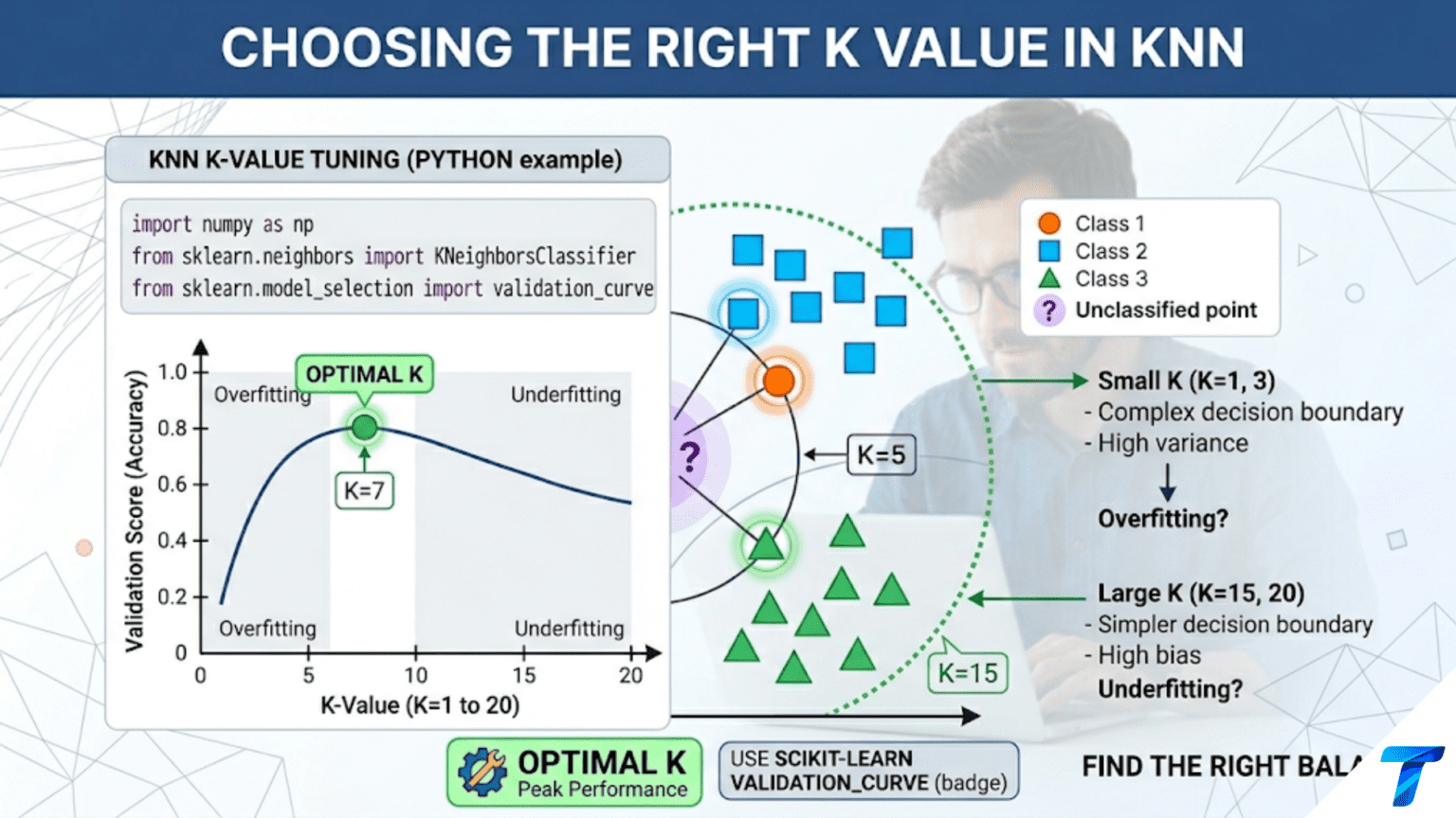
The optimal K in K-Nearest Neighbors is found by cross-validated grid search: train and evaluate the model at multiple K values, then select the K that maximizes validation performance. Small K values (K=1) produce complex, noisy decision boundaries that overfit; large K values produce overly smooth boundaries that underfit. The optimal K is typically found between K=3 and K=30 for most datasets, with cross-validation providing an unbiased estimate of where this sweet spot lies.
Introduction
Among the hyperparameters in machine learning, K in KNN has an unusually direct and interpretable effect on model behavior. Every increase in K smooths the decision boundary. Every decrease makes it more complex. There is no obscure internal mechanism — you can literally watch the boundary change by plotting it as K increases from 1 to 100.
This interpretability is a gift for understanding the bias-variance tradeoff. K=1 is the purest possible high-variance model: each prediction is determined entirely by the single nearest training point, memorizing the training set perfectly while generalizing poorly. K=N (all training samples) is the purest possible high-bias model: every prediction becomes the global majority class, ignoring all local structure. Somewhere between these extremes, your data has an optimal K.
Finding that K is not guesswork — it is a systematic process using cross-validation. This article covers every aspect of K selection: the theoretical tradeoffs, practical selection methods from simple cross-validation sweeps to statistically rigorous tests, common rules of thumb and when they fail, how K interacts with dataset size and dimensionality, and a complete Python implementation of the selection workflow.
The Bias-Variance Tradeoff Through the Lens of K
Before diving into selection methods, it helps to have precise intuition for what K controls.
K = 1: Maximum Variance, Zero Bias on Training Data
With K=1, each prediction is made solely by the single nearest training neighbor. This model has no training error — every training point is its own nearest neighbor, so it predicts every training label perfectly. But the decision boundary traces around every individual point, including mislabeled examples and outliers. On unseen data, performance suffers because the model has memorized noise rather than learned structure.
The variance of a K=1 classifier is high: small perturbations to the training set (adding or removing a few points, changing a few labels) can cause large changes to the decision boundary in regions near those points.
K = N: Maximum Bias, Minimum Variance
With K=N (using all training samples), every prediction is identical: the global majority class. This is the simplest possible predictor — it ignores all features entirely. The variance is zero (adding or removing a few training points will not change the global majority class). But bias is maximum: the model fails to capture any local structure.
The Optimal K: The Bias-Variance Sweet Spot
The optimal K minimizes total prediction error, which is the sum of bias² and variance:
As K increases from 1 to N:
- Bias increases: the model’s predictions become increasingly smoothed, losing local precision
- Variance decreases: each prediction averages more neighbors, becoming more stable
The optimal K sits at the bottom of the total error curve — where the benefit of lower variance no longer outweighs the cost of higher bias.
import numpy as np
import matplotlib.pyplot as plt
from sklearn.datasets import make_moons, make_classification
from sklearn.model_selection import StratifiedKFold, cross_val_score
from sklearn.neighbors import KNeighborsClassifier
from sklearn.preprocessing import StandardScaler
from sklearn.pipeline import Pipeline
import warnings
warnings.filterwarnings('ignore')


def visualize_k_effect(X, y, k_values=[1, 3, 7, 15, 30, 100], figsize=(18, 10)):
    """
    Visualize how decision boundaries change as K increases.
    Shows the bias-variance tradeoff directly.
    """
    scaler_v = StandardScaler()
    X_s = scaler_v.fit_transform(X)

    x_min, x_max = X_s[:, 0].min() - 0.5, X_s[:, 0].max() + 0.5
    y_min, y_max = X_s[:, 1].min() - 0.5, X_s[:, 1].max() + 0.5
    xx, yy = np.meshgrid(np.linspace(x_min, x_max, 250),
                          np.linspace(y_min, y_max, 250))
    grid = np.c_[xx.ravel(), yy.ravel()]

    n_cols = len(k_values)
    fig, axes = plt.subplots(1, n_cols, figsize=figsize)

    colors_cls = ['steelblue', 'coral']
    colors_bg  = ['#d0e8f8', '#fde8e0']

    for ax, k in zip(axes, k_values):
        knn_v = KNeighborsClassifier(n_neighbors=k)
        knn_v.fit(X_s, y)

        Z = knn_v.predict(grid).reshape(xx.shape)

        ax.contourf(xx, yy, Z, alpha=0.4,
                    colors=colors_bg[:len(np.unique(y))])
        ax.contour(xx, yy, Z, colors='black', linewidths=0.7, alpha=0.5)

        for cls_i, color in zip(np.unique(y), colors_cls):
            mask = y == cls_i
            ax.scatter(X_s[mask, 0], X_s[mask, 1],
                       c=color, edgecolors='white', s=35,
                       linewidth=0.4, alpha=0.85)

        train_acc = knn_v.score(X_s, y)
        ax.set_title(f'K = {k}\nTrain acc = {train_acc:.3f}',
                     fontsize=11, fontweight='bold')
        ax.set_xlabel('Feature 1', fontsize=9)
        ax.set_ylabel('Feature 2', fontsize=9)
        ax.grid(True, alpha=0.2)

        # Label the regime
        if k <= 2:
            regime = "Overfit"
            color_label = '#cc3333'
        elif k >= len(y) // 3:
            regime = "Underfit"
            color_label = '#3366cc'
        else:
            regime = "Balanced"
            color_label = '#33aa33'

        ax.text(0.05, 0.05, regime,
                transform=ax.transAxes, fontsize=10,
                color=color_label, fontweight='bold',
                bbox=dict(boxstyle='round', fc='white', alpha=0.8))

    plt.suptitle('Effect of K on KNN Decision Boundary\n'
                 '(Left = high variance/overfit → Right = high bias/underfit)',
                 fontsize=14, fontweight='bold', y=1.02)
    plt.tight_layout()
    plt.savefig('knn_k_effect_boundaries.png', dpi=150, bbox_inches='tight')
    plt.show()
    print("Saved: knn_k_effect_boundaries.png")


np.random.seed(42)
X_vis, y_vis = make_moons(n_samples=300, noise=0.25, random_state=42)
visualize_k_effect(X_vis, y_vis, k_values=[1, 3, 7, 15, 30, 100])Method 1: Cross-Validated Grid Search
The most reliable and general method for K selection is cross-validated grid search: evaluate the model at every candidate K value using cross-validation, and select the K with the best average validation score.
import numpy as np
import matplotlib.pyplot as plt
from sklearn.datasets import make_classification, load_wine, load_breast_cancer
from sklearn.model_selection import StratifiedKFold, cross_val_score, GridSearchCV
from sklearn.neighbors import KNeighborsClassifier
from sklearn.preprocessing import StandardScaler
from sklearn.pipeline import Pipeline


def knn_k_selection_cv(X, y, k_range=None, cv_folds=5, scoring='accuracy',
                         n_repeats=3, random_state=42):
    """
    Select optimal K for KNN using repeated stratified cross-validation.

    Args:
        X, y:         Features and labels
        k_range:      List/array of K values to try
        cv_folds:     Number of CV folds
        scoring:      Sklearn metric string
        n_repeats:    Number of CV repetitions for lower-variance estimates
        random_state: Random seed

    Returns:
        Dictionary with results, optimal K, and plot data
    """
    from sklearn.model_selection import RepeatedStratifiedKFold

    if k_range is None:
        n = len(y)
        k_range = list(range(1, min(31, n // cv_folds)))

    pipeline = Pipeline([
        ('scaler', StandardScaler()),
        ('knn',    KNeighborsClassifier())
    ])

    cv = RepeatedStratifiedKFold(n_splits=cv_folds, n_repeats=n_repeats,
                                  random_state=random_state)

    mean_scores = []
    std_scores  = []

    for k in k_range:
        pipeline.set_params(knn__n_neighbors=k)
        scores = cross_val_score(pipeline, X, y, cv=cv,
                                  scoring=scoring, n_jobs=-1)
        mean_scores.append(scores.mean())
        std_scores.append(scores.std())

    mean_scores = np.array(mean_scores)
    std_scores  = np.array(std_scores)
    best_idx    = np.argmax(mean_scores)
    best_k      = k_range[best_idx]
    best_score  = mean_scores[best_idx]

    return {
        'k_range':     np.array(k_range),
        'mean_scores': mean_scores,
        'std_scores':  std_scores,
        'best_k':      best_k,
        'best_score':  best_score,
        'best_idx':    best_idx,
    }


def plot_k_selection_curve(results, title='KNN: K Selection Curve',
                            figsize=(10, 6)):
    """
    Plot mean CV score ± 1 std across K values.
    Marks the optimal K and the '1-SE rule' K.
    """
    k_range  = results['k_range']
    means    = results['mean_scores']
    stds     = results['std_scores']
    best_k   = results['best_k']
    best_idx = results['best_idx']

    # 1-Standard Error Rule: select the largest K within 1 SE of the best
    # This prefers simpler (larger K) models when performance is statistically tied
    one_se_threshold = means[best_idx] - stds[best_idx]
    one_se_candidates = [k for k, m in zip(k_range, means) if m >= one_se_threshold]
    k_1se = max(one_se_candidates)  # Prefer largest K (simplest) within 1-SE

    fig, ax = plt.subplots(figsize=figsize)

    ax.plot(k_range, means, 'o-', color='steelblue',
            linewidth=2.5, markersize=7, label='CV score (mean)')
    ax.fill_between(k_range, means - stds, means + stds,
                    alpha=0.15, color='steelblue', label='±1 std')

    # Mark optimal K
    ax.axvline(x=best_k, color='coral', linestyle='--', lw=2,
               label=f'Best K = {best_k} (score={means[best_idx]:.4f})')

    # Mark 1-SE K (if different from best)
    if k_1se != best_k:
        ax.axvline(x=k_1se, color='mediumseagreen', linestyle=':', lw=2,
                   label=f'1-SE rule K = {k_1se} (simpler model)')

    # Mark 1-SE threshold
    ax.axhline(y=one_se_threshold, color='gray', linestyle=':', lw=1.5,
               alpha=0.6, label=f'1-SE threshold = {one_se_threshold:.4f}')

    ax.set_xlabel('K (Number of Neighbors)', fontsize=12)
    ax.set_ylabel(f'CV {results.get("scoring", "Score")}', fontsize=12)
    ax.set_title(f'{title}\n(Best K={best_k}, Score={means[best_idx]:.4f})',
                 fontsize=13, fontweight='bold')
    ax.legend(fontsize=10, loc='lower right')
    ax.grid(True, alpha=0.3)

    # Add text annotations for the regimes
    ax.axvspan(k_range[0], k_range[len(k_range)//4],
               alpha=0.04, color='red', label='_nolegend_')
    ax.axvspan(k_range[3*len(k_range)//4], k_range[-1],
               alpha=0.04, color='blue', label='_nolegend_')

    ax.text(k_range[1], ax.get_ylim()[0] + 0.01,
            'Overfit\nregion', fontsize=8, color='darkred', alpha=0.7)
    ax.text(k_range[-3], ax.get_ylim()[0] + 0.01,
            'Underfit\nregion', fontsize=8, color='darkblue', alpha=0.7,
            ha='right')

    plt.tight_layout()
    plt.savefig('knn_k_selection_curve.png', dpi=150)
    plt.show()
    print("Saved: knn_k_selection_curve.png")

    return best_k, k_1se


# Run on multiple datasets
datasets = {
    'Wine':          load_wine(),
    'Breast Cancer': load_breast_cancer(),
}

print("=== K Selection via Cross-Validation ===\n")

for name, data in datasets.items():
    results = knn_k_selection_cv(
        data.data, data.target,
        k_range=list(range(1, 41)),
        cv_folds=5, scoring='accuracy', n_repeats=3
    )
    results['scoring'] = 'Accuracy'

    best_k, k_1se = plot_k_selection_curve(
        results, title=f'KNN K-Selection: {name} Dataset'
    )

    print(f"\n  {name} Dataset:")
    print(f"    Samples: {len(data.target)}, Features: {data.data.shape[1]}")
    print(f"    Best K (max score):  K={results['best_k']}, "
          f"Score={results['best_score']:.4f}")
    print(f"    1-SE Rule K:         K={k_1se} (prefers simpler model)")
    print()
The 1-Standard Error Rule: Prefer Simpler Models
When multiple K values produce statistically indistinguishable performance, which should you choose? The 1-Standard Error Rule from Leo Breiman’s work on decision trees (later adapted broadly) provides a principled answer: select the simplest model whose performance is within 1 standard error of the best.
For KNN, “simpler” means larger K (smoother boundary, fewer effective parameters). The 1-SE rule therefore recommends the largest K whose mean CV score is at least as high as (best_score − best_std).
Why this makes sense:
A model at K=7 with CV score 0.912 ± 0.015 and a model at K=15 with CV score 0.908 ± 0.014 are not meaningfully different in performance. The difference (0.004) is well within the noise level (0.015). The K=15 model is simpler, will generalize more smoothly, and is less sensitive to noise near the boundary. Prefer it.
import numpy as np

def one_se_rule(k_range, mean_scores, std_scores):
    """
    Apply the 1-Standard Error Rule to select K.

    Returns the largest K whose mean score is within
    1 standard error of the best score.

    This prefers simpler (larger K, smoother) models
    when performance differences are not meaningful.
    """
    best_idx = np.argmax(mean_scores)
    threshold = mean_scores[best_idx] - std_scores[best_idx]

    # All K values where score >= threshold
    valid_ks = [k for k, score in zip(k_range, mean_scores)
                if score >= threshold]

    # Return the largest valid K (simplest model)
    return max(valid_ks)


def compare_k_selection_rules(X, y, k_range, cv_folds=10, random_state=42):
    """
    Compare different K selection rules on the same dataset.

    Rules compared:
    1. Maximum CV score (most common)
    2. 1-Standard Error Rule (prefer simpler)
    3. sqrt(n) rule of thumb
    4. Odd K closest to sqrt(n) (binary classification)
    """
    from sklearn.model_selection import RepeatedStratifiedKFold
    from sklearn.pipeline import Pipeline
    from sklearn.preprocessing import StandardScaler

    pipeline = Pipeline([
        ('scaler', StandardScaler()),
        ('knn', KNeighborsClassifier())
    ])

    cv = RepeatedStratifiedKFold(n_splits=cv_folds, n_repeats=5,
                                  random_state=random_state)

    mean_scores, std_scores = [], []
    for k in k_range:
        pipeline.set_params(knn__n_neighbors=k)
        sc = cross_val_score(pipeline, X, y, cv=cv, scoring='accuracy', n_jobs=-1)
        mean_scores.append(sc.mean())
        std_scores.append(sc.std())

    mean_scores = np.array(mean_scores)
    std_scores  = np.array(std_scores)

    n = len(y)

    # Rule 1: Maximum CV score
    k_max = k_range[np.argmax(mean_scores)]

    # Rule 2: 1-SE Rule
    k_1se = one_se_rule(k_range, mean_scores, std_scores)

    # Rule 3: sqrt(n)
    k_sqrt = int(np.round(np.sqrt(n)))
    k_sqrt = max(1, min(k_sqrt, max(k_range)))

    # Rule 4: Odd K nearest to sqrt(n) (reduces ties in binary classification)
    k_odd = k_sqrt if k_sqrt % 2 == 1 else k_sqrt + 1
    k_odd = min(k_odd, max(k_range))

    rules = {
        f'Max CV score':      k_max,
        f'1-SE Rule':         k_1se,
        f'sqrt(n)={k_sqrt}':  k_sqrt,
        f'Odd sqrt(n)':       k_odd,
    }

    print(f"  n={n}, sqrt(n)≈{np.sqrt(n):.1f}")
    print(f"\n  {'Rule':<25} | {'K':>4} | {'CV Score':>10} | {'Assessment'}")
    print("  " + "-" * 60)

    best_score = mean_scores[np.argmax(mean_scores)]
    for rule_name, k_val in rules.items():
        k_idx = list(k_range).index(k_val) if k_val in k_range else 0
        score = mean_scores[k_idx]
        within_1se = abs(score - best_score) <= std_scores[np.argmax(mean_scores)]
        flag = "✓ within 1-SE" if within_1se else "✗ outside 1-SE"
        print(f"  {rule_name:<25} | {k_val:>4} | {score:>10.4f} | {flag}")

    return rules, mean_scores, std_scores


np.random.seed(42)
X_rule, y_rule = make_classification(
    n_samples=600, n_features=15, n_informative=10, random_state=42
)
k_candidates = list(range(1, 51))

print("=== K Selection Rules Comparison ===\n")
rules, means, stds = compare_k_selection_rules(X_rule, y_rule, k_candidates)
Rules of Thumb: When to Use Them and When Not To
Several rules of thumb for choosing K appear frequently in the literature. Understanding their derivations helps you know when they apply.
The Square Root Rule: K ≈ √n
The most popular rule of thumb sets K ≈ √n, where n is the number of training samples. This emerges from an asymptotic analysis: under certain regularity conditions, the optimal K for minimizing mean squared error in KNN regression scales as O(n^(2/(d+2))), and for d=2 features this simplifies to approximately √n.
When it applies well: Balanced binary classification, moderate dimensionality (2–10 features), n in the hundreds to low thousands.
When it fails:
- High dimensionality: the optimal K grows more slowly in high dimensions
- Class imbalance: √n may select far too many neighbors when the minority class is sparse
- Small datasets: √(50) = 7, which is already a large fraction of total data
- Non-uniform data: when class density varies strongly across the feature space
import numpy as np
import matplotlib.pyplot as plt
from sklearn.datasets import make_classification
from sklearn.model_selection import cross_val_score, RepeatedStratifiedKFold
from sklearn.neighbors import KNeighborsClassifier
from sklearn.preprocessing import StandardScaler
from sklearn.pipeline import Pipeline

def evaluate_sqrt_rule(n_values, n_features=10, cv_folds=5, random_state=42):
    """
    Test how well the sqrt(n) rule tracks the true optimal K
    across different dataset sizes.
    """
    np.random.seed(random_state)

    results = []

    for n in n_values:
        X_n, y_n = make_classification(
            n_samples=n, n_features=n_features,
            n_informative=max(3, n_features // 2),
            random_state=random_state
        )

        k_sqrt = max(1, int(np.round(np.sqrt(n))))
        k_range = list(range(1, min(k_sqrt * 3 + 1, n // 5)))

        pipeline = Pipeline([
            ('scaler', StandardScaler()),
            ('knn', KNeighborsClassifier())
        ])

        cv = RepeatedStratifiedKFold(n_splits=cv_folds, n_repeats=3,
                                      random_state=random_state)

        mean_scores = []
        for k in k_range:
            pipeline.set_params(knn__n_neighbors=k)
            sc = cross_val_score(pipeline, X_n, y_n, cv=cv,
                                  scoring='accuracy', n_jobs=-1)
            mean_scores.append(sc.mean())

        k_true_best = k_range[np.argmax(mean_scores)]
        score_sqrt  = mean_scores[k_range.index(k_sqrt)] if k_sqrt in k_range else None
        score_best  = max(mean_scores)
        gap         = score_best - score_sqrt if score_sqrt else None

        results.append({
            'n':          n,
            'k_sqrt':     k_sqrt,
            'k_best':     k_true_best,
            'score_sqrt': score_sqrt,
            'score_best': score_best,
            'gap':        gap,
        })

    print("=== sqrt(n) Rule Evaluation ===\n")
    print(f"  {'n':>6} | {'√n':>5} | {'sqrt(n) K':>10} | {'True Best K':>12} | "
          f"{'Sqrt Score':>11} | {'Best Score':>11} | {'Gap':>6}")
    print("  " + "-" * 80)

    for r in results:
        gap_str = f"{r['gap']:.4f}" if r['gap'] is not None else "N/A"
        print(f"  {r['n']:>6,} | {np.sqrt(r['n']):>5.1f} | {r['k_sqrt']:>10} | "
              f"{r['k_best']:>12} | {r['score_sqrt']:>11.4f} | "
              f"{r['score_best']:>11.4f} | {gap_str:>6}")

    print("\n  Interpretation: Small gap = sqrt(n) rule works well here.")
    print("  Large gap = cross-validation would give better results.")


evaluate_sqrt_rule(n_values=[100, 300, 500, 1000, 2000, 5000])The Odd-K Rule for Binary Classification
When K is even, ties are possible: K/2 neighbors vote class 0, K/2 vote class 1. The algorithm must break the tie somehow — usually by defaulting to the smaller class index, which introduces an asymmetric bias. Using odd K eliminates ties entirely in binary classification.
import numpy as np
from sklearn.datasets import make_classification
from sklearn.model_selection import cross_val_score
from sklearn.neighbors import KNeighborsClassifier
from sklearn.preprocessing import StandardScaler
from sklearn.pipeline import Pipeline

def compare_odd_vs_even_k(X, y, k_pairs=None):
    """
    Compare adjacent odd and even K values to demonstrate
    tie-breaking effects in binary classification.
    """
    if k_pairs is None:
        k_pairs = [(2, 3), (4, 5), (6, 7), (8, 9), (10, 11), (14, 15), (20, 21)]

    pipeline = Pipeline([
        ('scaler', StandardScaler()),
        ('knn', KNeighborsClassifier())
    ])

    print("=== Odd vs Even K in Binary Classification ===\n")
    print(f"  {'K pair (even, odd)':>22} | {'Even K Score':>13} | "
          f"{'Odd K Score':>12} | {'Odd Better?':>11}")
    print("  " + "-" * 68)

    odd_better_count = 0
    for k_even, k_odd in k_pairs:
        pipeline.set_params(knn__n_neighbors=k_even)
        score_even = cross_val_score(
            pipeline, X, y, cv=5, scoring='accuracy', n_jobs=-1
        ).mean()

        pipeline.set_params(knn__n_neighbors=k_odd)
        score_odd = cross_val_score(
            pipeline, X, y, cv=5, scoring='accuracy', n_jobs=-1
        ).mean()

        odd_better = score_odd >= score_even
        if odd_better:
            odd_better_count += 1
        flag = "✓ Yes" if odd_better else "✗ No"
        print(f"  {'(' + str(k_even) + ', ' + str(k_odd) + ')':>22} | "
              f"{score_even:>13.4f} | {score_odd:>12.4f} | {flag:>11}")

    print(f"\n  Odd K outperformed: {odd_better_count}/{len(k_pairs)} comparisons")
    print("  Conclusion: Prefer odd K for binary classification to avoid ties.")


np.random.seed(42)
X_odd, y_odd = make_classification(
    n_samples=500, n_features=10, n_informative=6,
    n_classes=2, random_state=42
)

compare_odd_vs_even_k(X_odd, y_odd)Method 2: Grid Search with Scikit-learn
Scikit-learn’s GridSearchCV provides a clean, production-ready API for K selection with additional features: parallel evaluation, refit on best parameters, and direct integration with Pipelines.
import numpy as np
from sklearn.datasets import load_breast_cancer
from sklearn.model_selection import GridSearchCV, train_test_split
from sklearn.neighbors import KNeighborsClassifier
from sklearn.preprocessing import StandardScaler
from sklearn.pipeline import Pipeline
from sklearn.metrics import classification_report

# Load dataset and make holdout split
data = load_breast_cancer()
X_bc, y_bc = data.data, data.target

X_dev, X_hold, y_dev, y_hold = train_test_split(
    X_bc, y_bc, test_size=0.15, random_state=42, stratify=y_bc
)

print("=== GridSearchCV for K and Metric Selection ===\n")
print(f"  Dev set: {len(y_dev)} samples | Holdout: {len(y_hold)} samples\n")

# Pipeline: scaling + KNN
pipeline_gs = Pipeline([
    ('scaler', StandardScaler()),
    ('knn', KNeighborsClassifier())
])

# Parameter grid: K values + distance metrics + weighting schemes
param_grid = {
    'knn__n_neighbors': list(range(1, 31)),
    'knn__weights':     ['uniform', 'distance'],
    'knn__metric':      ['euclidean', 'manhattan'],
}

# 5-fold stratified cross-validation
from sklearn.model_selection import StratifiedKFold
cv_gs = StratifiedKFold(n_splits=5, shuffle=True, random_state=42)

grid_search = GridSearchCV(
    pipeline_gs,
    param_grid,
    cv=cv_gs,
    scoring='roc_auc',           # Use AUC for medical data
    n_jobs=-1,
    refit=True,                  # Refit best model on all dev data
    verbose=0,
    return_train_score=True
)

grid_search.fit(X_dev, y_dev)

print(f"  Best parameters found:")
for param, val in grid_search.best_params_.items():
    param_clean = param.replace('knn__', '')
    print(f"    {param_clean}: {val}")

print(f"\n  Best CV AUC: {grid_search.best_score_:.4f}")

# Evaluate best model on holdout (only once!)
best_model = grid_search.best_estimator_
from sklearn.metrics import roc_auc_score, accuracy_score
y_hold_proba = best_model.predict_proba(X_hold)[:, 1]
y_hold_pred  = best_model.predict(X_hold)

holdout_auc = roc_auc_score(y_hold, y_hold_proba)
holdout_acc = accuracy_score(y_hold, y_hold_pred)

print(f"\n  Holdout AUC:      {holdout_auc:.4f}")
print(f"  Holdout Accuracy: {holdout_acc:.4f}")
print(f"  CV-Holdout gap:   {grid_search.best_score_ - holdout_auc:+.4f}")

# Show top 10 parameter combinations
import pandas as pd

cv_results_df = pd.DataFrame(grid_search.cv_results_)
top_10 = (cv_results_df[['param_knn__n_neighbors',
                           'param_knn__weights',
                           'param_knn__metric',
                           'mean_test_score',
                           'std_test_score',
                           'mean_train_score']]
           .sort_values('mean_test_score', ascending=False)
           .head(10))

print(f"\n  Top 10 configurations by CV AUC:\n")
print(f"  {'K':>4} | {'Weights':>10} | {'Metric':>10} | "
      f"{'Test AUC':>9} | {'±':>7} | {'Train AUC':>9} | Overfit?")
print("  " + "-" * 72)

for _, row in top_10.iterrows():
    gap = row['mean_train_score'] - row['mean_test_score']
    flag = "⚠" if gap > 0.05 else ""
    print(f"  {int(row['param_knn__n_neighbors']):>4} | "
          f"{str(row['param_knn__weights']):>10} | "
          f"{str(row['param_knn__metric']):>10} | "
          f"{row['mean_test_score']:>9.4f} | "
          f"{row['std_test_score']:>7.4f} | "
f"{row['mean_train_score']:>9.4f} | {flag}")How K Interacts with Dataset Properties
The optimal K is not independent of your dataset. Several dataset properties shift the optimal K up or down.
Effect of Dataset Size
As n grows, the optimal K generally grows too (roughly as √n), but more slowly in high dimensions. The intuition: with more data, each neighborhood contains more points, so you can afford to expand K without losing resolution.
Effect of Class Imbalance
With severe class imbalance (e.g., 95% class 0, 5% class 1), the K nearest neighbors of any point will contain mostly class 0 examples — not necessarily because they are more similar, but because they are everywhere. This pushes the model to always predict class 0.
Mitigations: use weights='distance', reduce K (fewer neighbors = less dominated by majority class), or combine with oversampling.
import numpy as np
import matplotlib.pyplot as plt
from sklearn.datasets import make_classification
from sklearn.model_selection import cross_val_score, StratifiedKFold
from sklearn.neighbors import KNeighborsClassifier
from sklearn.preprocessing import StandardScaler
from sklearn.pipeline import Pipeline
from sklearn.metrics import make_scorer, f1_score

def analyze_k_vs_imbalance(prevalences, n_total=1000, k_range=None):
    """
    Show how class imbalance shifts the optimal K value.
    Uses F1 score (better for imbalanced data) rather than accuracy.
    """
    if k_range is None:
        k_range = list(range(1, 31))

    np.random.seed(42)
    f1_scorer = make_scorer(f1_score, zero_division=0)

    fig, axes = plt.subplots(1, len(prevalences), figsize=(16, 5))

    print("=== Optimal K vs Class Imbalance ===\n")
    print(f"  {'Prevalence':>12} | {'Optimal K (F1)':>15} | {'Best F1':>9}")
    print("  " + "-" * 42)

    for ax, prev in zip(axes, prevalences):
        X_imb, y_imb = make_classification(
            n_samples=n_total, n_features=10, n_informative=6,
            weights=[1 - prev, prev], random_state=42
        )

        pipeline = Pipeline([
            ('scaler', StandardScaler()),
            ('knn', KNeighborsClassifier())
        ])

        cv = StratifiedKFold(n_splits=5, shuffle=True, random_state=42)
        means = []

        for k in k_range:
            pipeline.set_params(knn__n_neighbors=k)
            sc = cross_val_score(pipeline, X_imb, y_imb,
                                  cv=cv, scoring=f1_scorer, n_jobs=-1)
            means.append(sc.mean())

        means = np.array(means)
        best_k = k_range[np.argmax(means)]

        ax.plot(k_range, means, 'o-', color='steelblue', lw=2, markersize=5)
        ax.axvline(x=best_k, color='coral', linestyle='--', lw=2,
                   label=f'Best K={best_k}')
        ax.set_title(f'Prevalence = {prev*100:.0f}%\nBest K = {best_k}',
                     fontsize=11, fontweight='bold')
        ax.set_xlabel('K', fontsize=10)
        ax.set_ylabel('CV F1 Score', fontsize=10)
        ax.legend(fontsize=9)
        ax.grid(True, alpha=0.3)

        print(f"  {prev*100:>11.0f}% | {best_k:>15} | {means.max():>9.4f}")

    plt.suptitle('Effect of Class Imbalance on Optimal K\n'
                 '(Severe imbalance requires lower K to preserve minority class signal)',
                 fontsize=13, fontweight='bold', y=1.02)
    plt.tight_layout()
    plt.savefig('knn_k_vs_imbalance.png', dpi=150, bbox_inches='tight')
    plt.show()
    print("\nSaved: knn_k_vs_imbalance.png")


analyze_k_vs_imbalance(prevalences=[0.40, 0.20, 0.10, 0.05])
Effect of Dimensionality
In high dimensions, the curse of dimensionality means that neighbors are not meaningfully “near.” Using small K in high dimensions amplifies this problem: the single nearest neighbor may be nearly as far away as a random point. Larger K provides some averaging that partially compensates, but the fundamental problem remains.
import numpy as np
from sklearn.datasets import make_classification
from sklearn.model_selection import cross_val_score, StratifiedKFold
from sklearn.neighbors import KNeighborsClassifier
from sklearn.preprocessing import StandardScaler
from sklearn.pipeline import Pipeline

def analyze_k_vs_dimensionality(feature_counts, n_informative_frac=0.5):
    """
    Show how the optimal K shifts with increasing dimensionality.
    """
    np.random.seed(42)
    n_total = 800
    k_range = list(range(1, 41))

    pipeline = Pipeline([
        ('scaler', StandardScaler()),
        ('knn', KNeighborsClassifier())
    ])

    cv = StratifiedKFold(n_splits=5, shuffle=True, random_state=42)

    print("=== Optimal K vs Feature Dimensionality ===\n")
    print(f"  {'Features':>10} | {'Informative':>12} | {'Optimal K':>10} | "
          f"{'Best Acc':>9} | Regime")
    print("  " + "-" * 58)

    optimal_ks = []

    for n_feat in feature_counts:
        n_info = max(3, int(n_feat * n_informative_frac))
        n_red  = min(n_feat - n_info, n_info)

        X_d, y_d = make_classification(
            n_samples=n_total, n_features=n_feat,
            n_informative=n_info, n_redundant=n_red,
            random_state=42
        )

        means = []
        for k in k_range:
            pipeline.set_params(knn__n_neighbors=k)
            sc = cross_val_score(pipeline, X_d, y_d,
                                  cv=cv, scoring='accuracy', n_jobs=-1)
            means.append(sc.mean())

        means = np.array(means)
        best_k = k_range[np.argmax(means)]
        optimal_ks.append(best_k)

        regime = ("Low-dim (KNN works well)" if n_feat <= 10
                  else "High-dim (KNN struggles)" if n_feat >= 50
                  else "Moderate")

        print(f"  {n_feat:>10} | {n_info:>12} | {best_k:>10} | "
              f"{means.max():>9.4f} | {regime}")

    print(f"\n  Pattern: Optimal K {'tends to increase' if optimal_ks[-1] > optimal_ks[0] else 'varies'} "
          f"with dimensionality.")
    print("  In very high dimensions, KNN performance degrades regardless of K.")
    print("  Consider PCA or feature selection before applying KNN.")


analyze_k_vs_dimensionality(feature_counts=[2, 5, 10, 20, 50, 100])Method 3: Learning Curve for K — Visualizing Bias-Variance Tradeoff
Rather than just reporting the optimal K, plotting the full training and validation score curves as K varies gives a visual diagnosis of the model’s behavior. This is the K-axis analogue of the training-size learning curve from Article 70.
import numpy as np
import matplotlib.pyplot as plt
from sklearn.datasets import make_classification
from sklearn.model_selection import StratifiedKFold, cross_val_score
from sklearn.neighbors import KNeighborsClassifier
from sklearn.preprocessing import StandardScaler
from sklearn.pipeline import Pipeline

def plot_k_bias_variance_curve(X, y, k_range=None, cv_folds=5,
                                 scoring='accuracy', title="KNN Bias-Variance Curve"):
    """
    Plot both training and validation scores as K varies.

    Shows the classic bias-variance picture:
    - Training score starts high (K=1 = perfect memorization) and falls
    - Validation score starts low, peaks, then falls
    - The gap between them quantifies overfitting at each K
    """
    if k_range is None:
        k_range = list(range(1, min(61, len(y) // cv_folds)))

    pipeline = Pipeline([
        ('scaler', StandardScaler()),
        ('knn', KNeighborsClassifier())
    ])

    cv = StratifiedKFold(n_splits=cv_folds, shuffle=True, random_state=42)

    train_means, train_stds = [], []
    val_means,   val_stds   = [], []

    from sklearn.model_selection import cross_validate
    for k in k_range:
        pipeline.set_params(knn__n_neighbors=k)
        result = cross_validate(
            pipeline, X, y, cv=cv, scoring=scoring,
            return_train_score=True, n_jobs=-1
        )
        train_means.append(result['train_score'].mean())
        train_stds.append(result['train_score'].std())
        val_means.append(result['test_score'].mean())
        val_stds.append(result['test_score'].std())

    train_means = np.array(train_means)
    val_means   = np.array(val_means)
    train_stds  = np.array(train_stds)
    val_stds    = np.array(val_stds)

    gaps = train_means - val_means
    best_val_idx = np.argmax(val_means)
    best_k = k_range[best_val_idx]

    fig, (ax1, ax2) = plt.subplots(2, 1, figsize=(11, 9), sharex=True)

    # Top: training and validation scores
    ax1.plot(k_range, train_means, 'o-', color='steelblue', lw=2.5,
             markersize=5, label='Training score')
    ax1.fill_between(k_range, train_means - train_stds,
                     train_means + train_stds, alpha=0.12, color='steelblue')

    ax1.plot(k_range, val_means, 's-', color='coral', lw=2.5,
             markersize=5, label='Validation score (CV)')
    ax1.fill_between(k_range, val_means - val_stds,
                     val_means + val_stds, alpha=0.12, color='coral')

    ax1.axvline(x=best_k, color='black', linestyle='--', lw=1.8,
                label=f'Best K = {best_k}')
    ax1.set_ylabel(scoring.replace('_', ' ').title(), fontsize=11)
    ax1.set_title(f'{title}\n(Best K={best_k}, Val={val_means[best_val_idx]:.4f})',
                  fontsize=12, fontweight='bold')
    ax1.legend(fontsize=10)
    ax1.grid(True, alpha=0.3)

    # Annotate regimes
    ax1.text(k_range[1], ax1.get_ylim()[0] + 0.01,
             'Overfit\n(high variance)', fontsize=8, color='darkred',
             ha='left', alpha=0.7)
    ax1.text(k_range[-3], ax1.get_ylim()[0] + 0.01,
             'Underfit\n(high bias)', fontsize=8, color='darkblue',
             ha='right', alpha=0.7)

    # Bottom: gap between training and validation (overfitting degree)
    ax2.fill_between(k_range, gaps, 0, where=(gaps >= 0),
                     alpha=0.3, color='coral', label='Train-Val gap (overfit)')
    ax2.plot(k_range, gaps, '-', color='coral', lw=2)
    ax2.axvline(x=best_k, color='black', linestyle='--', lw=1.8)
    ax2.axhline(y=0, color='gray', lw=1, alpha=0.5)
    ax2.set_xlabel('K (Number of Neighbors)', fontsize=11)
    ax2.set_ylabel('Train - Val Gap', fontsize=11)
    ax2.set_title('Overfitting Degree by K\n(Large gap = memorizing, small gap = generalizing)',
                  fontsize=11, fontweight='bold')
    ax2.legend(fontsize=10)
    ax2.grid(True, alpha=0.3)

    plt.tight_layout()
    plt.savefig('knn_bias_variance_curve.png', dpi=150)
    plt.show()
    print("Saved: knn_bias_variance_curve.png")

    # Print summary table for key K values
    print(f"\n  Key K values summary:")
    print(f"  {'K':>4} | {'Train':>8} | {'Val':>8} | {'Gap':>7} | {'Regime'}")
    print("  " + "-" * 48)

    highlight_ks = [1, 3, 5, best_k] + k_range[::max(1, len(k_range)//6)]
    highlight_ks = sorted(set(highlight_ks))

    for k in highlight_ks:
        if k in k_range:
            idx = k_range.index(k)
            gap = gaps[idx]
            if gap > 0.15:
                regime = "High variance"
            elif gap < 0.02 and val_means[idx] < val_means[best_val_idx] - 0.05:
                regime = "High bias"
            elif idx == best_val_idx:
                regime = "★ OPTIMAL"
            else:
                regime = "Balanced"
            print(f"  {k:>4} | {train_means[idx]:>8.4f} | {val_means[idx]:>8.4f} | "
                  f"{gap:>7.4f} | {regime}")

    return best_k, val_means[best_val_idx]


np.random.seed(42)
X_bv, y_bv = make_classification(
    n_samples=600, n_features=12, n_informative=8, random_state=42
)

plot_k_bias_variance_curve(X_bv, y_bv, k_range=list(range(1, 61)),
                            scoring='accuracy',
title="KNN Bias-Variance Tradeoff Curve")Method 4: Statistical Significance Testing Between K Values
When two K values produce very similar cross-validation scores, you might wonder whether the difference is real or just sampling noise. Paired t-tests on CV fold scores provide a principled answer.
import numpy as np
from scipy import stats
from sklearn.datasets import make_classification
from sklearn.model_selection import StratifiedKFold
from sklearn.neighbors import KNeighborsClassifier
from sklearn.preprocessing import StandardScaler
from sklearn.pipeline import Pipeline

def compare_k_values_statistically(X, y, k_values_to_compare,
                                     cv_folds=10, random_state=42):
    """
    Use paired t-test to determine if differences between K values
    are statistically significant.

    Since all models are evaluated on the same folds, fold-level
    scores are paired — the variance within each fold cancels out,
    giving much more statistical power than unpaired tests.

    Args:
        k_values_to_compare: List of K values to compare pairwise
        cv_folds:            Number of folds (more = better powered test)
    """
    pipeline = Pipeline([
        ('scaler', StandardScaler()),
        ('knn', KNeighborsClassifier())
    ])

    cv = StratifiedKFold(n_splits=cv_folds, shuffle=True, random_state=random_state)

    # Collect per-fold scores for each K
    fold_scores = {}
    for k in k_values_to_compare:
        pipeline.set_params(knn__n_neighbors=k)
        scores = []
        for train_idx, val_idx in cv.split(X, y):
            from sklearn.preprocessing import StandardScaler as SS
            import copy
            p = copy.deepcopy(pipeline)
            p.fit(X[train_idx], y[train_idx])
            scores.append(p.score(X[val_idx], y[val_idx]))
        fold_scores[k] = np.array(scores)

    print("=== Statistical Comparison of K Values ===\n")
    print(f"  {'K':>4} | {'Mean Acc':>10} | {'Std':>7}")
    print("  " + "-" * 27)
    for k in k_values_to_compare:
        print(f"  {k:>4} | {fold_scores[k].mean():>10.4f} | {fold_scores[k].std():>7.4f}")

    print(f"\n  Pairwise paired t-tests (α=0.05):\n")
    print(f"  {'K1 vs K2':>12} | {'Δ Mean':>8} | {'t-stat':>8} | {'p-value':>9} | {'Significant?':>13} | {'Prefer'}")
    print("  " + "-" * 75)

    for i, k1 in enumerate(k_values_to_compare):
        for k2 in k_values_to_compare[i+1:]:
            diff = fold_scores[k1] - fold_scores[k2]
            t_stat, p_val = stats.ttest_rel(fold_scores[k1], fold_scores[k2])
            significant = p_val < 0.05
            delta = fold_scores[k1].mean() - fold_scores[k2].mean()

            if significant:
                prefer = f"K={k1}" if delta > 0 else f"K={k2}"
            else:
                prefer = f"K={max(k1,k2)} (simpler)"  # Prefer larger K if tied

            sig_str = "✓ Yes" if significant else "✗ No (tied)"
            print(f"  {str(k1)+'vs'+str(k2):>12} | {delta:>+8.4f} | {t_stat:>8.3f} | "
                  f"{p_val:>9.4f} | {sig_str:>13} | {prefer}")

    print(f"\n  Interpretation:")
    print(f"  Non-significant difference → no evidence to prefer one K over the other.")
    print(f"  Apply 1-SE rule: pick the larger K (simpler model) among tied candidates.")


np.random.seed(42)
X_stat, y_stat = make_classification(
    n_samples=500, n_features=10, n_informative=7, random_state=42
)

compare_k_values_statistically(
    X_stat, y_stat,
    k_values_to_compare=[5, 7, 9, 11, 15, 20],
    cv_folds=10
)Complete K Selection Workflow
Putting all methods together into a single, reusable workflow:
import numpy as np
import matplotlib.pyplot as plt
from sklearn.datasets import load_wine
from sklearn.model_selection import (
    train_test_split, GridSearchCV, StratifiedKFold,
    cross_val_score, RepeatedStratifiedKFold
)
from sklearn.neighbors import KNeighborsClassifier
from sklearn.preprocessing import StandardScaler
from sklearn.pipeline import Pipeline
from sklearn.metrics import roc_auc_score, accuracy_score, f1_score

def full_knn_k_selection_workflow(X, y, dataset_name="Dataset",
                                   holdout_size=0.15,
                                   k_min=1, k_max=50,
                                   cv_folds=5, cv_repeats=5,
                                   random_state=42):
    """
    Complete, production-quality K selection workflow.

    Steps:
    1. Reserve holdout test set (touch only at the very end)
    2. Cross-validated K sweep on development set
    3. Apply 1-SE rule to prefer simpler model
    4. Optionally expand to grid search over metrics and weights
    5. Evaluate final model on holdout (once)
    6. Report full diagnostic

    Args:
        X, y:           Features and labels
        dataset_name:   For display
        holdout_size:   Fraction for final test set
        k_min, k_max:   Range of K values to search
        cv_folds:       Number of cross-validation folds
        cv_repeats:     Number of CV repetitions
        random_state:   Random seed
    """
    print(f"{'='*60}")
    print(f"  KNN K-Selection Workflow: {dataset_name}")
    print(f"{'='*60}")
    print(f"\n  Dataset: {len(y):,} samples, {X.shape[1]} features, "
          f"{len(np.unique(y))} classes")

    # Step 1: Holdout split
    X_dev, X_hold, y_dev, y_hold = train_test_split(
        X, y, test_size=holdout_size, random_state=random_state, stratify=y
    )
    print(f"  Dev: {len(y_dev):,} | Holdout: {len(y_hold):,}\n")

    # Step 2: K sweep on dev set
    pipeline = Pipeline([
        ('scaler', StandardScaler()),
        ('knn', KNeighborsClassifier())
    ])

    k_range = list(range(k_min, min(k_max + 1, len(y_dev) // cv_folds)))
    cv = RepeatedStratifiedKFold(n_splits=cv_folds, n_repeats=cv_repeats,
                                  random_state=random_state)

    print("  Step 2: K sweep (cross-validation)")
    mean_scores, std_scores = [], []

    for k in k_range:
        pipeline.set_params(knn__n_neighbors=k)
        sc = cross_val_score(pipeline, X_dev, y_dev, cv=cv,
                              scoring='accuracy', n_jobs=-1)
        mean_scores.append(sc.mean())
        std_scores.append(sc.std())

    mean_scores = np.array(mean_scores)
    std_scores  = np.array(std_scores)

    # Step 3: Apply selection rules
    best_idx  = np.argmax(mean_scores)
    k_best    = k_range[best_idx]
    score_best = mean_scores[best_idx]

    # 1-SE rule
    threshold = score_best - std_scores[best_idx]
    k_1se = max(k for k, s in zip(k_range, mean_scores) if s >= threshold)

    # sqrt(n) rule
    k_sqrt = max(1, int(round(np.sqrt(len(y_dev)))))
    k_sqrt = min(k_sqrt, max(k_range))
    # Make odd for binary classification
    if len(np.unique(y)) == 2 and k_sqrt % 2 == 0:
        k_sqrt_odd = k_sqrt + 1
    else:
        k_sqrt_odd = k_sqrt

    print(f"\n  {'Rule':<25} | {'K':>4} | {'CV Score':>9}")
    print("  " + "-" * 42)
    for rule_name, k_val in [
        ('Max CV score',       k_best),
        ('1-SE Rule',          k_1se),
        ('sqrt(n) rule',       k_sqrt),
        ('Odd sqrt(n)',        k_sqrt_odd),
    ]:
        k_idx = list(k_range).index(k_val) if k_val in k_range else 0
        score = mean_scores[k_idx]
        print(f"  {rule_name:<25} | {k_val:>4} | {score:>9.4f}")

    # Step 4: Final model using recommended K (1-SE rule)
    recommended_k = k_1se
    print(f"\n  Recommended K (1-SE rule): {recommended_k}")

    # Step 5: Evaluate on holdout
    best_pipeline = Pipeline([
        ('scaler', StandardScaler()),
        ('knn', KNeighborsClassifier(n_neighbors=recommended_k,
                                      weights='distance'))
    ])
    best_pipeline.fit(X_dev, y_dev)

    y_hold_pred  = best_pipeline.predict(X_hold)
    holdout_acc  = accuracy_score(y_hold, y_hold_pred)
    holdout_f1   = f1_score(y_hold, y_hold_pred, average='weighted')

    cv_score_at_k = mean_scores[list(k_range).index(recommended_k)]

    print(f"\n  Step 5: Final Holdout Evaluation (first and only look)")
    print(f"  {'Metric':<20} | {'CV Estimate':>12} | {'Holdout':>8} | Gap")
    print("  " + "-" * 52)
    print(f"  {'Accuracy':<20} | {cv_score_at_k:>12.4f} | {holdout_acc:>8.4f} | "
          f"{holdout_acc - cv_score_at_k:+.4f}")
    print(f"  {'F1 (weighted)':<20} | {'N/A':>12} | {holdout_f1:>8.4f} | N/A")

    # Plot K selection curve
    fig, ax = plt.subplots(figsize=(10, 6))
    ax.plot(k_range, mean_scores, 'o-', color='steelblue', lw=2.5,
            markersize=6, label='CV Accuracy (mean)')
    ax.fill_between(k_range, mean_scores - std_scores,
                    mean_scores + std_scores, alpha=0.15, color='steelblue')
    ax.axvline(x=k_best, color='coral', linestyle='--', lw=2,
               label=f'Best K={k_best} (acc={score_best:.4f})')
    ax.axvline(x=k_1se, color='mediumseagreen', linestyle=':', lw=2,
               label=f'1-SE K={k_1se} (simpler, recommended)')
    ax.axhline(y=threshold, color='gray', linestyle=':', lw=1.5, alpha=0.7,
               label=f'1-SE threshold = {threshold:.4f}')
    ax.set_xlabel('K (Number of Neighbors)', fontsize=12)
    ax.set_ylabel('CV Accuracy', fontsize=12)
    ax.set_title(f'{dataset_name}: K Selection Curve\n'
                 f'(Recommended K={recommended_k}, Holdout Acc={holdout_acc:.4f})',
                 fontsize=12, fontweight='bold')
    ax.legend(fontsize=10, loc='lower right')
    ax.grid(True, alpha=0.3)
    plt.tight_layout()
    plt.savefig(f'knn_k_selection_{dataset_name.replace(" ", "_")}.png', dpi=150)
    plt.show()
    print(f"\n  Saved: knn_k_selection_{dataset_name.replace(' ', '_')}.png")

    return {
        'recommended_k': recommended_k,
        'k_best':        k_best,
        'k_1se':         k_1se,
        'cv_score':      cv_score_at_k,
        'holdout_acc':   holdout_acc,
    }


# Run on Wine dataset
wine = load_wine()
results_wine = full_knn_k_selection_workflow(
    wine.data, wine.target,
    dataset_name="Wine Dataset",
    k_min=1, k_max=40,
    cv_folds=5, cv_repeats=5
)Common Mistakes in K Selection
Mistake 1: Testing K on the test set The most harmful mistake. If you try K=1, 3, 5, … 30, evaluate each on your test set, and pick the best, you have effectively trained K on the test set. The reported performance will be optimistically biased. Always use cross-validation on the training/development set for K selection.
Mistake 2: Using accuracy as the sole metric on imbalanced data With 95% class 0 prevalence, K=500 that always predicts class 0 achieves 95% accuracy. Use F1, AUC, or recall/precision depending on your cost asymmetry. The optimal K under accuracy and under F1 can differ dramatically on imbalanced data.
Mistake 3: Forgetting to normalize K selection results measured on unnormalized features are meaningless — the features with larger magnitudes dominate distance calculations entirely. Always scale before searching K.
Mistake 4: Setting K without considering n K=50 on a dataset with 100 training samples means each prediction averages over 50% of all training data. This is usually extreme oversmoothing. As a sanity check, K should generally be much smaller than n — at most 10–15% of training size.
Mistake 5: Not trying odd K values for binary classification When your optimal K sweep returns an even value, try the adjacent odd values. They eliminate tie-breaking randomness and often perform marginally better or equally.
import numpy as np

def k_selection_sanity_checks(k_recommended, n_train, n_classes):
    """
    Run sanity checks on a recommended K value.
    """
    print("=== K Selection Sanity Checks ===\n")
    issues = []

    # Check 1: K relative to training size
    k_pct = k_recommended / n_train * 100
    if k_pct > 20:
        issues.append(f"K={k_recommended} is {k_pct:.1f}% of training set — likely oversmoothing")
    elif k_pct < 0.5:
        issues.append(f"K={k_recommended} is very small relative to {n_train} training samples — high variance risk")

    # Check 2: Odd K for binary classification
    if n_classes == 2 and k_recommended % 2 == 0:
        issues.append(f"K={k_recommended} is even for binary classification — ties possible, try K={k_recommended+1}")

    # Check 3: K=1 special case
    if k_recommended == 1:
        issues.append("K=1 is the highest-variance setting — consider if this truly generalizes or just memorizes")

    # Check 4: Very large K
    if k_recommended > 50:
        issues.append(f"K={k_recommended} is very large — verify the model isn't just predicting the majority class")

    print(f"  Recommended K:   {k_recommended}")
    print(f"  Training size:   {n_train:,}")
    print(f"  K / n:           {k_pct:.2f}%")
    print(f"  Classes:         {n_classes}")

    if issues:
        print(f"\n  ⚠ Issues detected:")
        for issue in issues:
            print(f"    - {issue}")
    else:
        print(f"\n  ✓ No issues detected — K={k_recommended} looks reasonable")

# Test on several scenarios
print("Scenario 1: Reasonable K")
k_selection_sanity_checks(k_recommended=7, n_train=300, n_classes=2)
print("\nScenario 2: Even K for binary")
k_selection_sanity_checks(k_recommended=10, n_train=300, n_classes=2)
print("\nScenario 3: Very large K")
k_selection_sanity_checks(k_recommended=80, n_train=300, n_classes=3)Summary
Choosing K in KNN is one of the clearest examples of the bias-variance tradeoff in practice. Every increase in K increases bias and reduces variance; the optimal K is where their sum is minimized for your specific dataset.
Cross-validated grid search is the most reliable K selection method. Running it across a range from K=1 to √n or 2√n, using repeated stratified K-fold for stability, and applying the 1-SE rule to prefer simpler (larger K) models when performance differences are statistically negligible — this workflow produces good K choices consistently across diverse datasets.
Rules of thumb like K ≈ √n provide useful starting points but should be treated as hypotheses to test, not final answers. The optimal K depends on dataset size, dimensionality, class balance, and noise level in ways that no simple formula captures perfectly.
A few habits pay dividends every time: always scale features before searching K, use F1 or AUC rather than accuracy for imbalanced data, prefer odd K for binary classification, and never evaluate K selection performance on your holdout test set.