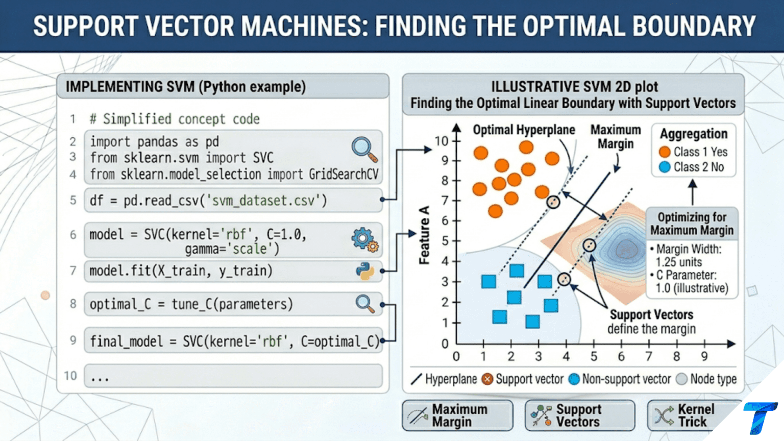
A Support Vector Machine (SVM) finds the decision boundary that maximizes the margin — the distance between the boundary and the nearest training points from each class. Those nearest points are called support vectors, and the optimal boundary is determined entirely by them. This maximum-margin principle produces classifiers that generalize well even in high-dimensional spaces, because it finds the most “room” between classes rather than just any separating line.
Introduction
Every classification algorithm draws a boundary between classes. Logistic regression finds the boundary that best fits the training data by maximizing likelihood. Decision trees partition the feature space by greedily minimizing impurity. Neural networks shape increasingly complex boundaries through stacked transformations. But Support Vector Machines ask a fundamentally different question: among all possible boundaries that correctly separate the classes, which one generalizes best to new data?
The SVM’s answer is elegant: the best boundary is the one with the maximum margin — the widest possible gap between the boundary and the training points of each class. A boundary that passes through a narrow corridor of training points will be fragile; tiny perturbations in the data or new observations that fall in that corridor would be misclassified. A boundary with a wide margin is robust — it separates classes with the most “room to spare.”
This geometrically motivated principle leads to a precise mathematical optimization problem, a beautiful connection to convex duality, and an algorithmic trick — the kernel trick — that makes SVMs effective in spaces with thousands or millions of dimensions where the classes may not be linearly separable at all.
This article builds a complete understanding of SVMs from first principles: the geometric intuition of margins and support vectors, the hard-margin and soft-margin formulations, practical implementation with scikit-learn, the kernel trick preview, and a thorough comparison of SVMs with other classifiers.
The Core Idea: Maximizing the Margin
Linear Separability and Hyperplanes
For two-class problems with linearly separable data, infinitely many hyperplanes (lines in 2D, planes in 3D, hyperplanes in higher dimensions) correctly separate the classes. The question is which one to choose.
A hyperplane in d-dimensional space is defined by:
where w is the weight vector (normal to the hyperplane) and b is the bias. Points on one side satisfy wᵀx + b > 0 (class +1), and points on the other side satisfy wᵀx + b < 0 (class −1).
The distance from a point x to this hyperplane is:
The Margin
The margin of a separating hyperplane is the total distance between the two parallel hyperplanes that just touch the nearest points from each class:
The SVM finds the hyperplane that maximizes this margin — equivalently, minimizes ‖w‖. The points that lie exactly on the margin boundaries (at distance 1/‖w‖ from the decision boundary) are the support vectors — they are the only training points that determine the solution.
import numpy as np
import matplotlib.pyplot as plt
from sklearn.svm import SVC
from sklearn.datasets import make_classification, make_blobs
from sklearn.preprocessing import StandardScaler
from sklearn.model_selection import train_test_split
import warnings
warnings.filterwarnings('ignore')

np.random.seed(42)


def visualize_svm_margin(X, y, title="SVM: Maximum Margin Classifier",
                          figsize=(12, 7)):
    """
    Visualize the SVM decision boundary, margin, and support vectors.

    Highlights:
    - Decision boundary (solid line)
    - Margin boundaries (dashed lines)
    - Support vectors (circled)
    - Margin width annotation
    """
    # Fit linear SVM
    scaler = StandardScaler()
    X_scaled = scaler.fit_transform(X)

    svm = SVC(kernel='linear', C=1e6)  # Large C → near hard-margin
    svm.fit(X_scaled, y)

    # Plot setup
    x_min = X_scaled[:, 0].min() - 0.8
    x_max = X_scaled[:, 0].max() + 0.8
    y_min = X_scaled[:, 1].min() - 0.8
    y_max = X_scaled[:, 1].max() + 0.8

    xx, yy = np.meshgrid(np.linspace(x_min, x_max, 300),
                          np.linspace(y_min, y_max, 300))
    Z = svm.decision_function(np.c_[xx.ravel(), yy.ravel()])
    Z = Z.reshape(xx.shape)

    fig, ax = plt.subplots(figsize=figsize)

    # Decision regions (faint background coloring)
    ax.contourf(xx, yy, Z, levels=[-np.inf, 0, np.inf],
                colors=['#ffd0d0', '#d0e8ff'], alpha=0.3)

    # Decision boundary and margin boundaries
    ax.contour(xx, yy, Z, levels=[-1, 0, 1],
               colors=['coral', 'black', 'steelblue'],
               linestyles=['--', '-', '--'],
               linewidths=[2, 2.5, 2])

    # Training points
    colors = ['coral', 'steelblue']
    markers = ['o', 's']
    class_labels = ['Class −1', 'Class +1']
    for cls_i, (color, marker, label) in enumerate(zip(colors, markers, class_labels)):
        mask = y == np.unique(y)[cls_i]
        ax.scatter(X_scaled[mask, 0], X_scaled[mask, 1],
                   c=color, marker=marker, s=80,
                   edgecolors='white', linewidth=0.8,
                   label=label, zorder=4)

    # Highlight support vectors
    sv_idx = svm.support_
    ax.scatter(X_scaled[sv_idx, 0], X_scaled[sv_idx, 1],
               s=200, facecolors='none', edgecolors='black',
               linewidth=2.5, zorder=5, label='Support Vectors')

    # Margin width annotation
    w = svm.coef_[0]
    margin = 2 / np.linalg.norm(w)

    # Draw arrow showing margin
    # Find a point on the decision boundary
    if abs(w[1]) > 1e-10:
        x0 = 0
        y0 = -svm.intercept_[0] / w[1]
        # Direction perpendicular to boundary
        perp = np.array([w[0], w[1]]) / np.linalg.norm(w)
        start = np.array([x0, y0]) - perp / np.linalg.norm(w)
        end   = np.array([x0, y0]) + perp / np.linalg.norm(w)

        ax.annotate('', xy=end, xytext=start,
                    arrowprops=dict(arrowstyle='<->', color='darkgreen',
                                    lw=2, mutation_scale=15))
        mid = (start + end) / 2
        ax.text(mid[0] + 0.15, mid[1],
                f'Margin = {margin:.2f}',
                color='darkgreen', fontsize=11, fontweight='bold')

    ax.set_xlim(x_min, x_max)
    ax.set_ylim(y_min, y_max)
    ax.set_xlabel('Feature 1 (scaled)', fontsize=12)
    ax.set_ylabel('Feature 2 (scaled)', fontsize=12)
    ax.set_title(f'{title}\n'
                 f'Support vectors: {len(sv_idx)} | '
                 f'Margin width: {margin:.3f}',
                 fontsize=12, fontweight='bold')
    ax.legend(fontsize=10, loc='upper left')
    ax.grid(True, alpha=0.2)

    # Dashed line labels
    ax.text(x_max - 0.1, ax.get_ylim()[0] + 0.15,
            '← Margin boundary (class −1)',
            ha='right', fontsize=9, color='coral', style='italic')
    ax.text(x_min + 0.1, ax.get_ylim()[1] - 0.15,
            'Margin boundary (class +1) →',
            ha='left', fontsize=9, color='steelblue', style='italic')

    plt.tight_layout()
    plt.savefig('svm_margin_visualization.png', dpi=150, bbox_inches='tight')
    plt.show()
    print("Saved: svm_margin_visualization.png")

    print(f"\n  SVM Results:")
    print(f"    Support vectors: {len(sv_idx)} "
          f"(of {len(y)} training points)")
    print(f"    Margin width:    {margin:.4f}")
    print(f"    Weight vector:   [{w[0]:.4f}, {w[1]:.4f}]")
    print(f"    Bias:            {svm.intercept_[0]:.4f}")
    print(f"\n  Key insight: Only {len(sv_idx)} points determine the entire solution.")
    print(f"  Remove any non-support-vector point → same boundary.")
    print(f"  Move a support vector → boundary shifts.")


# Create linearly separable dataset
X_sep, y_sep = make_blobs(n_samples=80, centers=2, cluster_std=0.7,
                            random_state=42)
y_sep_pm = np.where(y_sep == 0, -1, 1)  # Convert to ±1 labels

visualize_svm_margin(X_sep, y_sep_pm,
"SVM: Maximum Margin Decision Boundary")Why Maximizing Margin Works
The margin can be understood as a measure of confidence. A new test point that falls far from the decision boundary — deep into the margin of its predicted class — is being classified with high confidence. A point that barely crosses the boundary is classified with low confidence.
Maximizing the margin is equivalent to maximizing the minimum confidence over all training points. By theory (VC dimension bounds and PAC learning), a larger margin corresponds to lower model complexity and better generalization bounds, even when the number of features is very large.
The Hard-Margin SVM: Formal Optimization
For linearly separable data, the SVM solves:
The objective minimizes ‖w‖² (equivalent to maximizing the margin 2/‖w‖). The constraints enforce that every training point is on the correct side of its margin boundary with at least unit distance.
This is a convex quadratic programming problem — a bowl-shaped objective with linear constraints. It has a unique global minimum and can be solved efficiently. The Lagrangian dual formulation, which is used in practice, transforms this into:
where α_i are the Lagrange multipliers. The key property of this dual: only support vectors have α_i > 0. This sparsity is why SVMs are efficient at prediction — only support vectors matter.
import numpy as np
from sklearn.svm import SVC
from sklearn.datasets import make_blobs
from sklearn.preprocessing import StandardScaler

np.random.seed(42)


def demonstrate_support_vector_sparsity(X, y, C_values=[0.1, 1.0, 10.0, 1000.0]):
    """
    Show how the number of support vectors changes with C (regularization).
    More support vectors = more complex boundary = potentially more overfit.

    In the hard-margin limit (C → ∞), only the truly borderline points
    become support vectors.
    """
    scaler = StandardScaler()
    X_s = scaler.fit_transform(X)

    print("=== Support Vector Sparsity vs C ===\n")
    print(f"  n_train = {len(y)}\n")
    print(f"  {'C':>8} | {'n_SVs':>7} | {'% of data':>10} | {'Train Acc':>10} | Interpretation")
    print("  " + "-" * 68)

    for C in C_values:
        svm = SVC(kernel='linear', C=C)
        svm.fit(X_s, y)
        n_sv   = len(svm.support_)
        pct_sv = n_sv / len(y) * 100
        tr_acc = svm.score(X_s, y)

        if C < 0.5:
            interp = "High regularization (wide margin, many SVs)"
        elif C < 5:
            interp = "Balanced"
        elif C < 100:
            interp = "Low regularization (tight margin, few SVs)"
        else:
            interp = "Hard-margin limit (minimum SVs)"

        print(f"  {C:>8.1f} | {n_sv:>7} | {pct_sv:>10.1f}% | "
              f"{tr_acc:>10.4f} | {interp}")

    print("\n  Insight: Smaller C = wider margin = more training points")
    print("  become support vectors (tolerate more violations).")
    print("  Larger C = narrower margin = fewer but more critical SVs.")


X_sparse, y_sparse = make_blobs(n_samples=120, centers=2, cluster_std=0.9,
                                  random_state=42)
demonstrate_support_vector_sparsity(X_sparse, y_sparse)The Soft-Margin SVM: Handling Non-Separable Data
Real datasets are rarely linearly separable. Noise, outliers, and overlapping class distributions mean that no hyperplane perfectly separates the classes. The soft-margin SVM extends the hard-margin formulation by allowing some training points to violate the margin, penalized by a cost parameter C.
The soft-margin optimization introduces slack variables ξ_i ≥ 0:
The C parameter controls the bias-variance tradeoff:
- Small C: Allows many violations — wide margin, high bias, low variance (underfitting)
- Large C: Allows few violations — narrow margin, low bias, high variance (overfitting)
import numpy as np
import matplotlib.pyplot as plt
from sklearn.svm import SVC
from sklearn.datasets import make_classification
from sklearn.preprocessing import StandardScaler
from sklearn.model_selection import train_test_split, cross_val_score


def visualize_soft_margin_c_effect(X, y, C_values, figsize=(20, 5)):
    """
    Show how C controls the margin width and boundary complexity.
    Side-by-side plots for multiple C values.
    """
    scaler = StandardScaler()
    X_s = scaler.fit_transform(X)

    x_min = X_s[:, 0].min() - 0.5
    x_max = X_s[:, 0].max() + 0.5
    y_min_v = X_s[:, 1].min() - 0.5
    y_max_v = X_s[:, 1].max() + 0.5

    xx, yy = np.meshgrid(np.linspace(x_min, x_max, 250),
                          np.linspace(y_min_v, y_max_v, 250))

    n_cols = len(C_values)
    fig, axes = plt.subplots(1, n_cols, figsize=figsize)

    colors_bg  = ['#ffd0d0', '#d0e8ff']
    colors_pts = ['coral', 'steelblue']

    for ax, C in zip(axes, C_values):
        svm = SVC(kernel='linear', C=C)
        svm.fit(X_s, y)

        Z = svm.decision_function(np.c_[xx.ravel(), yy.ravel()])
        Z = Z.reshape(xx.shape)

        ax.contourf(xx, yy, Z, levels=[-np.inf, 0, np.inf],
                    colors=colors_bg, alpha=0.3)
        ax.contour(xx, yy, Z, levels=[-1, 0, 1],
                   colors=['coral', 'black', 'steelblue'],
                   linestyles=['--', '-', '--'], linewidths=[1.5, 2, 1.5])

        for cls_i, color in enumerate(colors_pts):
            mask = y == np.unique(y)[cls_i]
            ax.scatter(X_s[mask, 0], X_s[mask, 1], c=color,
                       s=50, edgecolors='white', linewidth=0.5,
                       alpha=0.85, zorder=3)

        # Highlight support vectors
        sv = svm.support_
        ax.scatter(X_s[sv, 0], X_s[sv, 1], s=180,
                   facecolors='none', edgecolors='black',
                   linewidth=2, zorder=4)

        # Margin width
        w = svm.coef_[0]
        margin = 2 / np.linalg.norm(w)
        n_sv   = len(sv)

        regime = ("Underfit\n(C too small)" if C <= 0.01
                  else "Overfit\n(C too large)" if C >= 100
                  else "Balanced")

        ax.set_title(f'C = {C}\n'
                     f'Margin = {margin:.2f} | SVs = {n_sv}\n{regime}',
                     fontsize=10, fontweight='bold')
        ax.set_xlabel('Feature 1', fontsize=9)
        ax.set_xlim(x_min, x_max); ax.set_ylim(y_min_v, y_max_v)
        ax.grid(True, alpha=0.2)

    axes[0].set_ylabel('Feature 2', fontsize=9)
    plt.suptitle('Soft-Margin SVM: Effect of C on Margin Width and Complexity\n'
                 '(Small C = wide margin/underfit → Large C = narrow margin/overfit)',
                 fontsize=12, fontweight='bold', y=1.02)
    plt.tight_layout()
    plt.savefig('svm_soft_margin_c.png', dpi=150, bbox_inches='tight')
    plt.show()
    print("Saved: svm_soft_margin_c.png")


np.random.seed(42)
X_soft, y_soft = make_classification(
    n_samples=150, n_features=2, n_informative=2,
    n_redundant=0, n_clusters_per_class=1,
    class_sep=0.8, random_state=42
)
y_soft_pm = np.where(y_soft == 0, -1, 1)

visualize_soft_margin_c_effect(
    X_soft, y_soft_pm,
    C_values=[0.01, 0.1, 1.0, 10.0, 100.0]
)


def tune_c_with_crossvalidation(X, y, C_range=None, cv=5):
    """
    Select optimal C using cross-validation.
    Both too-small and too-large C hurt generalization.
    """
    if C_range is None:
        C_range = np.logspace(-3, 3, 25)

    scaler = StandardScaler()
    X_s = scaler.fit_transform(X)

    cv_scores = []
    for C in C_range:
        svm = SVC(kernel='linear', C=C)
        scores = cross_val_score(svm, X_s, y, cv=cv, scoring='accuracy')
        cv_scores.append(scores.mean())

    cv_scores  = np.array(cv_scores)
    best_C     = C_range[np.argmax(cv_scores)]
    best_score = cv_scores.max()

    fig, ax = plt.subplots(figsize=(10, 5))
    ax.semilogx(C_range, cv_scores, 'o-', color='steelblue', lw=2.5,
                markersize=7)
    ax.axvline(x=best_C, color='coral', linestyle='--', lw=2,
               label=f'Best C = {best_C:.3f} (acc={best_score:.4f})')
    ax.set_xlabel('C (log scale)', fontsize=12)
    ax.set_ylabel(f'{cv}-Fold CV Accuracy', fontsize=12)
    ax.set_title('SVM C Hyperparameter Tuning\n'
                 '(Too small = underfit, too large = overfit)',
                 fontsize=12, fontweight='bold')
    ax.legend(fontsize=10); ax.grid(True, alpha=0.3)
    plt.tight_layout()
    plt.savefig('svm_c_tuning.png', dpi=150)
    plt.show()
    print("Saved: svm_c_tuning.png")

    print(f"\n  C selection results:")
    print(f"    Best C:    {best_C:.4f}")
    print(f"    Best CV acc: {best_score:.4f}")
    print(f"\n  Note: C interacts with feature scale — always scale features")
    print(f"  before tuning C. An unscaled feature with range [0, 1000] vs")
    print(f"  one with range [0, 1] will dominate the margin calculation.")
    return best_C


best_C = tune_c_with_crossvalidation(X_soft, y_soft_pm)Hinge Loss: The SVM’s Objective from an ML Perspective
The SVM optimization can also be written as an empirical risk minimization with hinge loss plus L2 regularization:
where f(x) = wᵀx + b and λ = 1/C controls regularization strength.
The hinge loss max(0, 1 − y·f(x)) is zero when the prediction is correct with sufficient confidence (y·f(x) ≥ 1), and grows linearly otherwise. This gives SVMs their characteristic robustness to outliers compared with logistic regression’s log loss, which grows logarithmically for correct predictions.
import numpy as np
import matplotlib.pyplot as plt


def compare_loss_functions():
    """
    Compare hinge loss (SVM), logistic loss, and 0-1 loss.
    Shows why SVMs are margin-based and how hinge loss creates sparsity.
    """
    yf = np.linspace(-3, 3, 500)  # y * f(x): margin

    hinge_loss   = np.maximum(0, 1 - yf)
    logistic_loss = np.log(1 + np.exp(-yf)) / np.log(2)  # Normalized to bits
    zero_one_loss = (yf < 0).astype(float)

    fig, axes = plt.subplots(1, 2, figsize=(14, 5))

    ax = axes[0]
    ax.plot(yf, hinge_loss,   color='steelblue',      lw=2.5, label='Hinge (SVM)')
    ax.plot(yf, logistic_loss, color='coral',          lw=2.5, label='Logistic (log loss)')
    ax.plot(yf, zero_one_loss, color='mediumseagreen', lw=2.5,
            linestyle='--', label='0-1 loss (ideal, non-convex)')

    ax.axvline(x=0, color='gray', lw=1, alpha=0.5, linestyle=':')
    ax.axvline(x=1, color='steelblue', lw=1, alpha=0.5, linestyle=':',
               label='Margin boundary (y·f=1)')

    ax.fill_between(yf, hinge_loss, 0,
                    where=(yf >= 1), alpha=0.08, color='steelblue',
                    label='Zero hinge loss (within margin)')

    ax.set_xlabel('y · f(x)  [margin]', fontsize=12)
    ax.set_ylabel('Loss', fontsize=12)
    ax.set_title('Loss Function Comparison\n'
                 'Hinge loss = 0 when y·f(x) ≥ 1 (correct with margin)',
                 fontsize=11, fontweight='bold')
    ax.set_xlim(-3, 3); ax.set_ylim(-0.1, 3)
    ax.legend(fontsize=9); ax.grid(True, alpha=0.3)

    # Gradient comparison
    ax = axes[1]
    hinge_grad    = np.where(yf < 1, -1, 0)
    logistic_grad = -1 / (1 + np.exp(yf))

    ax.plot(yf, hinge_grad,    color='steelblue', lw=2.5, label='Hinge gradient')
    ax.plot(yf, logistic_grad, color='coral',     lw=2.5, label='Logistic gradient')
    ax.axvline(x=0, color='gray', lw=1, alpha=0.5, linestyle=':')
    ax.axvline(x=1, color='steelblue', lw=1, alpha=0.5, linestyle=':')
    ax.set_xlabel('y · f(x)  [margin]', fontsize=12)
    ax.set_ylabel('Loss gradient', fontsize=12)
    ax.set_title('Gradient Comparison\n'
                 'Hinge gradient is exactly 0 for well-classified points\n'
                 '→ sparsity and efficiency',
                 fontsize=11, fontweight='bold')
    ax.legend(fontsize=9); ax.grid(True, alpha=0.3)

    plt.suptitle('SVM Hinge Loss vs Logistic Regression Log Loss',
                 fontsize=13, fontweight='bold')
    plt.tight_layout()
    plt.savefig('svm_hinge_loss.png', dpi=150)
    plt.show()
    print("Saved: svm_hinge_loss.png")

    print("\n  Key differences:")
    print("  Hinge loss:")
    print("    • Exactly 0 for well-classified points (y·f(x) ≥ 1)")
    print("    • Gradient is exactly 0 → sparse solution via support vectors")
    print("    • Linear growth for violated points → robust to outliers")
    print("  Logistic loss:")
    print("    • Always positive, approaches 0 asymptotically")
    print("    • Non-zero gradient everywhere → all points influence boundary")
    print("    • Logarithmic growth → slightly more sensitive to outliers")


compare_loss_functions()Why Feature Scaling is Critical for SVMs
The SVM margin depends on the Euclidean distance in feature space. If features have very different scales — one ranges [0, 1], another [0, 1000] — the distance metric is dominated by the large-scale feature. The margin will then be almost entirely determined by the large-scale feature, effectively ignoring all others.
import numpy as np
from sklearn.svm import SVC
from sklearn.preprocessing import StandardScaler
from sklearn.model_selection import cross_val_score
from sklearn.datasets import load_breast_cancer

cancer = load_breast_cancer()
X_ca, y_ca = cancer.data, cancer.target

print("=== Why Feature Scaling Matters for SVMs ===\n")
print(f"  Breast Cancer dataset: {X_ca.shape[1]} features\n")
print(f"  Feature scale range:")
print(f"    Min range (max-min): {(X_ca.max(axis=0) - X_ca.min(axis=0)).min():.4f}")
print(f"    Max range (max-min): {(X_ca.max(axis=0) - X_ca.min(axis=0)).max():.4f}")
print(f"    Ratio: {(X_ca.max(axis=0) - X_ca.min(axis=0)).max() / (X_ca.max(axis=0) - X_ca.min(axis=0)).min():.1f}×\n")

svm_base = SVC(kernel='rbf', C=1.0)
scaler = StandardScaler()
X_scaled = scaler.fit_transform(X_ca)
svm_scaled = SVC(kernel='rbf', C=1.0)

scores_unscaled = cross_val_score(svm_base, X_ca, y_ca, cv=5)
scores_scaled   = cross_val_score(svm_scaled, X_scaled, y_ca, cv=5)

print(f"  {'Configuration':<30} | {'Mean Acc':>10} | {'Std':>7}")
print("  " + "-" * 50)
print(f"  {'SVM (no scaling)':<30} | {scores_unscaled.mean():>10.4f} | "
      f"{scores_unscaled.std():>7.4f}")
print(f"  {'SVM (StandardScaler)':<30} | {scores_scaled.mean():>10.4f} | "
      f"{scores_scaled.std():>7.4f}")

improvement = scores_scaled.mean() - scores_unscaled.mean()
print(f"\n  Accuracy improvement from scaling: {improvement*100:+.2f}%")
print(f"  Always scale features before training an SVM.")
print(f" Use StandardScaler (zero mean, unit variance) or MinMaxScaler.")SVM for Multi-Class Classification
The standard SVM formulation is binary. Multi-class classification is handled by decomposition strategies:
One-vs-Rest (OvR): Train one SVM per class (k SVMs for k classes). Each SVM distinguishes one class from all others. Classify by choosing the class whose SVM produces the highest decision function value.
One-vs-One (OvO): Train one SVM for every pair of classes (k(k-1)/2 SVMs). Classify by majority vote. This is scikit-learn’s default for SVC because it is faster to train (each SVM only sees two classes) and often more accurate.
import numpy as np
from sklearn.svm import SVC, LinearSVC
from sklearn.datasets import load_iris, load_wine
from sklearn.model_selection import cross_val_score, StratifiedKFold
from sklearn.preprocessing import StandardScaler
from sklearn.pipeline import Pipeline
from sklearn.multiclass import OneVsRestClassifier, OneVsOneClassifier


def multiclass_svm_comparison(X, y, class_names, dataset_name):
    """
    Compare OvR and OvO strategies for multi-class SVM.
    """
    pipeline_ovo = Pipeline([
        ('scaler', StandardScaler()),
        ('svm', SVC(kernel='rbf', C=1.0, decision_function_shape='ovo'))
    ])
    pipeline_ovr = Pipeline([
        ('scaler', StandardScaler()),
        ('svm', SVC(kernel='rbf', C=1.0, decision_function_shape='ovr'))
    ])
    pipeline_linear_ovr = Pipeline([
        ('scaler', StandardScaler()),
        ('svm', LinearSVC(C=1.0, max_iter=5000))
    ])

    cv = StratifiedKFold(n_splits=5, shuffle=True, random_state=42)

    strategies = {
        'RBF SVM (OvO, default)': pipeline_ovo,
        'RBF SVM (OvR)':          pipeline_ovr,
        'Linear SVM (OvR)':       pipeline_linear_ovr,
    }

    n_classes = len(np.unique(y))
    n_ovo = n_classes * (n_classes - 1) // 2
    n_ovr = n_classes

    print(f"=== Multi-Class SVM: {dataset_name} ===\n")
    print(f"  {n_classes} classes → OvO: {n_ovo} SVMs | OvR: {n_ovr} SVMs\n")
    print(f"  {'Strategy':<30} | {'Mean Acc':>10} | {'Std':>7}")
    print("  " + "-" * 50)

    for name, pipe in strategies.items():
        scores = cross_val_score(pipe, X, y, cv=cv, scoring='accuracy')
        print(f"  {name:<30} | {scores.mean():>10.4f} | {scores.std():>7.4f}")


wine = load_wine()
multiclass_svm_comparison(
    wine.data, wine.target, wine.target_names, "Wine Dataset"
)

iris = load_iris()
multiclass_svm_comparison(
    iris.data, iris.target, iris.target_names, "Iris Dataset"
)Comparing SVM with Other Classifiers
SVMs occupy a specific niche in the classifier landscape. Understanding their strengths and limitations relative to alternatives — logistic regression, decision trees, Random Forests, and k-NN — guides which algorithm to reach for first.
import numpy as np
from sklearn.svm import SVC
from sklearn.linear_model import LogisticRegression
from sklearn.tree import DecisionTreeClassifier
from sklearn.ensemble import RandomForestClassifier
from sklearn.neighbors import KNeighborsClassifier
from sklearn.datasets import (load_breast_cancer, load_wine,
                               make_classification, make_moons)
from sklearn.model_selection import RepeatedStratifiedKFold, cross_val_score
from sklearn.preprocessing import StandardScaler
from sklearn.pipeline import Pipeline


def comprehensive_classifier_comparison(datasets, cv_folds=5, cv_repeats=3):
    """
    Compare SVM against major classifier families across datasets.
    """
    classifiers = {
        'Logistic Regression':  Pipeline([('s', StandardScaler()),
                                           ('m', LogisticRegression(max_iter=1000))]),
        'Decision Tree':        DecisionTreeClassifier(random_state=42),
        'Random Forest':        RandomForestClassifier(n_estimators=100, random_state=42,
                                                         n_jobs=-1),
        'KNN (k=7)':            Pipeline([('s', StandardScaler()),
                                           ('m', KNeighborsClassifier(n_neighbors=7))]),
        'SVM Linear':           Pipeline([('s', StandardScaler()),
                                           ('m', SVC(kernel='linear', C=1.0))]),
        'SVM RBF':              Pipeline([('s', StandardScaler()),
                                           ('m', SVC(kernel='rbf', C=1.0, gamma='scale'))]),
    }

    cv = RepeatedStratifiedKFold(n_splits=cv_folds, n_repeats=cv_repeats,
                                  random_state=42)

    print("=== Classifier Comparison Across Datasets ===\n")

    for ds_name, (X, y) in datasets.items():
        print(f"  {ds_name} (n={len(y)}, d={X.shape[1]}):")
        print(f"  {'Classifier':<22} | {'Mean Acc':>10} | {'Std':>7}")
        print("  " + "-" * 43)

        scores_all = {}
        for clf_name, clf in classifiers.items():
            scores = cross_val_score(clf, X, y, cv=cv,
                                      scoring='accuracy', n_jobs=-1)
            scores_all[clf_name] = scores.mean()
            best = " ★" if scores.mean() == max(
                cross_val_score(c, X, y, cv=cv, scoring='accuracy', n_jobs=-1).mean()
                for c in classifiers.values()
            ) else ""
            print(f"  {clf_name:<22} | {scores.mean():>10.4f} | "
                  f"{scores.std():>7.4f}{best}")
        print()


datasets_comp = {
    'Breast Cancer':   (load_breast_cancer().data, load_breast_cancer().target),
    'Wine':            (load_wine().data,           load_wine().target),
    'Moons (noise=.2)': make_moons(400, noise=0.20, random_state=42),
    'High-Dim 50D':    make_classification(600, 50, n_informative=15,
                                           random_state=42),
}

comprehensive_classifier_comparison(datasets_comp)When SVMs Shine
SVMs tend to excel in these scenarios:
High-dimensional, low-sample settings. When d >> n (many features, few samples), SVMs often outperform ensemble methods. The kernel trick implicitly operates in very high-dimensional spaces, and the maximum-margin principle provides theoretical generalization guarantees that scale with the margin rather than the dimensionality.
Text classification. TF-IDF or bag-of-words features produce very high-dimensional sparse vectors. Linear SVMs handle these efficiently with LinearSVC, which scales to hundreds of thousands of features.
Clear but possibly nonlinear boundaries. The RBF kernel can capture circular or elliptical boundaries that logistic regression misses, while being more interpretable than deep neural networks.
When SVMs Struggle
Large datasets. The standard SVM solver has O(n²) to O(n³) time complexity in the number of training samples. For n > 50,000, training becomes slow. LinearSVC (which uses a faster solver) scales better but only for linear kernels.
Noisy, overlapping classes. When no clear margin exists, C tuning becomes critical and the advantage over logistic regression diminishes.
Multi-class problems with many classes. OvO requires k(k-1)/2 binary SVMs. For 100 classes, that is 4,950 SVMs — expensive to train and store.
SVM Decision Boundaries: A Visual Summary
import numpy as np
import matplotlib.pyplot as plt
from sklearn.svm import SVC
from sklearn.preprocessing import StandardScaler
from sklearn.datasets import make_moons, make_circles, make_classification


def compare_svm_kernels_visual(figsize=(18, 12)):
    """
    Visualize SVM boundaries with different kernels on four synthetic datasets.
    Shows when linear SVM is sufficient vs when kernels are needed.
    """
    np.random.seed(42)
    datasets = {
        'Linearly Separable':   make_classification(200, 2, n_informative=2,
                                                     n_redundant=0,
                                                     class_sep=2, random_state=42),
        'Two Moons':            make_moons(200, noise=0.15, random_state=42),
        'Concentric Circles':   make_circles(200, noise=0.10, factor=0.5,
                                              random_state=42),
        'XOR Pattern':          None,  # Will generate below
    }

    # XOR pattern
    X_xor = np.random.randn(200, 2)
    y_xor = np.logical_xor(X_xor[:, 0] > 0, X_xor[:, 1] > 0).astype(int)
    datasets['XOR Pattern'] = (X_xor, y_xor)

    kernels = ['linear', 'rbf', 'poly']
    kernel_labels = ['Linear SVM', 'RBF SVM', 'Polynomial SVM (deg=3)']
    kernel_params = [
        {'kernel': 'linear', 'C': 1.0},
        {'kernel': 'rbf',    'C': 1.0, 'gamma': 'scale'},
        {'kernel': 'poly',   'C': 1.0, 'degree': 3, 'gamma': 'scale'},
    ]

    n_rows = len(datasets)
    n_cols = len(kernels)
    fig, axes = plt.subplots(n_rows, n_cols, figsize=figsize)

    for row, (ds_name, (X, y)) in enumerate(datasets.items()):
        scaler = StandardScaler()
        X_s = scaler.fit_transform(X)

        x_min = X_s[:, 0].min() - 0.5
        x_max = X_s[:, 0].max() + 0.5
        y_min = X_s[:, 1].min() - 0.5
        y_max = X_s[:, 1].max() + 0.5
        xx, yy = np.meshgrid(np.linspace(x_min, x_max, 200),
                              np.linspace(y_min, y_max, 200))

        for col, (params, k_label) in enumerate(zip(kernel_params, kernel_labels)):
            ax = axes[row, col]
            svm = SVC(**params)
            svm.fit(X_s, y)

            Z = svm.predict(np.c_[xx.ravel(), yy.ravel()]).reshape(xx.shape)
            acc = svm.score(X_s, y)

            ax.contourf(xx, yy, Z, alpha=0.3,
                        colors=['#ffd0d0', '#d0e8ff'])
            ax.contour(xx, yy, Z, colors='black', linewidths=0.8, alpha=0.4)

            for cls_i, color in enumerate(['coral', 'steelblue']):
                mask = y == cls_i
                ax.scatter(X_s[mask, 0], X_s[mask, 1], c=color,
                           s=30, edgecolors='white', linewidth=0.4, alpha=0.85)

            sv = svm.support_
            ax.scatter(X_s[sv, 0], X_s[sv, 1], s=120,
                       facecolors='none', edgecolors='black', linewidth=1.5)

            if row == 0:
                ax.set_title(k_label, fontsize=11, fontweight='bold', pad=10)

            ax.set_ylabel(ds_name if col == 0 else '', fontsize=9, fontweight='bold')
            ax.set_xticks([]); ax.set_yticks([])

            color_acc = '#22aa22' if acc > 0.95 else ('#aaaa22' if acc > 0.85 else '#aa2222')
            ax.text(0.02, 0.02, f'Acc={acc:.2f}',
                    transform=ax.transAxes, fontsize=8,
                    color=color_acc, fontweight='bold',
                    bbox=dict(boxstyle='round', fc='white', alpha=0.8))

    plt.suptitle('SVM Kernels on Different Dataset Geometries\n'
                 '(Circles = support vectors, outlined points)',
                 fontsize=14, fontweight='bold', y=1.01)
    plt.tight_layout()
    plt.savefig('svm_kernel_comparison.png', dpi=150, bbox_inches='tight')
    plt.show()
    print("Saved: svm_kernel_comparison.png")


compare_svm_kernels_visual()SVR: Support Vector Regression
The SVM framework extends naturally to regression through Support Vector Regression (SVR). Instead of finding the widest margin between two classes, SVR finds the narrowest tube (epsilon-insensitive zone) that contains the majority of training points, with deviations beyond ε penalized.
The SVR objective:
subject to residuals |y_i − f(x_i)| ≤ ε + ξ_i (slack variables for points outside the tube).
The ε parameter defines the tube width — predictions within ε of the true value incur zero loss. This makes SVR robust to small noise in the target variable.
import numpy as np
import matplotlib.pyplot as plt
from sklearn.svm import SVR
from sklearn.preprocessing import StandardScaler
from sklearn.pipeline import Pipeline
from sklearn.model_selection import cross_val_score
from sklearn.datasets import fetch_california_housing


def demonstrate_svr(epsilon_values=[0.1, 0.5, 1.0]):
    """
    Show how epsilon controls the SVR tube width and support vector count.
    """
    np.random.seed(42)
    # Synthetic 1D regression
    X_1d = np.sort(np.random.uniform(0, 6, 120)).reshape(-1, 1)
    y_1d = np.sin(X_1d.ravel()) + 0.3 * np.random.randn(120)

    x_plot = np.linspace(0, 6, 300).reshape(-1, 1)

    fig, axes = plt.subplots(1, len(epsilon_values), figsize=(15, 5), sharey=True)

    for ax, eps in zip(axes, epsilon_values):
        svr = Pipeline([
            ('scaler', StandardScaler()),
            ('svr',    SVR(kernel='rbf', C=1.0, epsilon=eps))
        ])
        svr.fit(X_1d, y_1d)
        y_pred = svr.predict(x_plot)

        # Support vectors (points outside the tube)
        scaler_fit = svr.named_steps['scaler']
        svr_fit    = svr.named_steps['svr']
        X_s = scaler_fit.transform(X_1d)
        sv_idx = svr_fit.support_

        ax.scatter(X_1d, y_1d, color='steelblue', s=20, alpha=0.5, label='Data')
        ax.plot(x_plot, y_pred, 'coral', lw=2.5, label='SVR prediction')
        ax.fill_between(x_plot.ravel(),
                        y_pred - eps, y_pred + eps,
                        alpha=0.2, color='coral', label=f'ε-tube (±{eps})')
        ax.scatter(X_1d[sv_idx], y_1d[sv_idx],
                   s=80, facecolors='none', edgecolors='black',
                   linewidth=2, zorder=4, label=f'SVs ({len(sv_idx)})')
        ax.set_title(f'ε = {eps}\n{len(sv_idx)} support vectors',
                     fontsize=11, fontweight='bold')
        ax.set_xlabel('X', fontsize=10)
        ax.legend(fontsize=8, loc='upper right')
        ax.grid(True, alpha=0.2)

    axes[0].set_ylabel('y', fontsize=10)
    plt.suptitle('SVR: Effect of ε on Tube Width and Support Vectors\n'
                 'Larger ε = wider tube = fewer support vectors = simpler model',
                 fontsize=13, fontweight='bold')
    plt.tight_layout()
    plt.savefig('svr_epsilon_effect.png', dpi=150)
    plt.show()
    print("Saved: svr_epsilon_effect.png")


demonstrate_svr()


def svr_vs_other_regressors():
    """
    Compare SVR against linear regression and Random Forest Regressor
    on California Housing.
    """
    from sklearn.linear_model import Ridge
    from sklearn.ensemble import RandomForestRegressor

    housing = fetch_california_housing()
    X_h, y_h = housing.data, housing.target

    regressors = {
        'Ridge Regression':  Pipeline([('s', StandardScaler()), ('m', Ridge())]),
        'SVR (RBF)':         Pipeline([('s', StandardScaler()),
                                        ('m', SVR(kernel='rbf', C=10.0,
                                                   epsilon=0.1, gamma='scale'))]),
        'SVR (Linear)':      Pipeline([('s', StandardScaler()),
                                        ('m', SVR(kernel='linear', C=1.0))]),
        'Random Forest':     RandomForestRegressor(n_estimators=100,
                                                    random_state=42, n_jobs=-1),
    }

    print("=== SVR vs Other Regressors: California Housing ===\n")
    print(f"  {'Model':<22} | {'CV R²':>9} | {'CV RMSE':>9}")
    print("  " + "-" * 44)

    for name, reg in regressors.items():
        r2_scores   = cross_val_score(reg, X_h, y_h, cv=5,
                                       scoring='r2', n_jobs=-1)
        rmse_scores = np.sqrt(-cross_val_score(
            reg, X_h, y_h, cv=5,
            scoring='neg_mean_squared_error', n_jobs=-1
        ))
        print(f"  {name:<22} | {r2_scores.mean():>9.4f} | "
              f"{rmse_scores.mean():>9.4f}")

    print("\n  Note: SVR is competitive on smaller datasets but slower")
    print("  than Random Forest on large datasets (n > 10,000).")


svr_vs_other_regressors()
Probability Calibration for SVMs
By default, SVC does not output calibrated probabilities. When probability=True, it uses Platt scaling — fitting a sigmoid to the decision function values on held-out cross-validation folds. This post-hoc calibration is sometimes imperfect, and the calibration curve reveals whether the SVM’s probabilities match observed frequencies.
import numpy as np
import matplotlib.pyplot as plt
from sklearn.svm import SVC
from sklearn.linear_model import LogisticRegression
from sklearn.ensemble import RandomForestClassifier
from sklearn.calibration import calibration_curve, CalibratedClassifierCV
from sklearn.datasets import load_breast_cancer
from sklearn.model_selection import train_test_split
from sklearn.preprocessing import StandardScaler
from sklearn.pipeline import Pipeline


def compare_calibration(X_train, y_train, X_test, y_test):
    """
    Compare probability calibration across SVM, SVM+Platt, LR, and RF.
    """
    models = {
        'Logistic Regression':   Pipeline([('s', StandardScaler()),
                                            ('m', LogisticRegression())]),
        'SVM (no calibration)':  Pipeline([('s', StandardScaler()),
                                            ('m', SVC(probability=True))]),
        'SVM + Platt Scaling':   Pipeline([
            ('s', StandardScaler()),
            ('m', CalibratedClassifierCV(SVC(), method='sigmoid', cv=5))
        ]),
        'Random Forest':         RandomForestClassifier(n_estimators=100,
                                                          random_state=42,
                                                          n_jobs=-1),
    }

    fig, ax = plt.subplots(figsize=(9, 7))
    ax.plot([0, 1], [0, 1], 'k--', lw=1.5, alpha=0.5,
            label='Perfect calibration')

    colors = ['steelblue', 'coral', 'mediumseagreen', 'mediumpurple']

    for (name, model), color in zip(models.items(), colors):
        model.fit(X_train, y_train)
        y_prob = model.predict_proba(X_test)[:, 1]
        prob_true, prob_pred = calibration_curve(y_test, y_prob, n_bins=10)
        ax.plot(prob_pred, prob_true, 'o-', color=color, lw=2,
                markersize=7, label=name)

    ax.set_xlabel('Mean predicted probability', fontsize=12)
    ax.set_ylabel('Fraction of positives', fontsize=12)
    ax.set_title('Probability Calibration Curves\n'
                 'Closer to diagonal = better calibrated probabilities',
                 fontsize=12, fontweight='bold')
    ax.legend(fontsize=9); ax.grid(True, alpha=0.3)
    plt.tight_layout()
    plt.savefig('svm_calibration.png', dpi=150)
    plt.show()
    print("Saved: svm_calibration.png")

    print("\n  When calibrated probabilities matter (risk scores, medical):")
    print("  1. Use SVM + Platt scaling or isotonic regression")
    print("  2. Or use Logistic Regression which is naturally well-calibrated")
    print("  3. Evaluate calibration with a calibration curve, not just accuracy")


cancer = load_breast_cancer()
X_ca, y_ca = cancer.data, cancer.target
X_tr_ca, X_te_ca, y_tr_ca, y_te_ca = train_test_split(
    X_ca, y_ca, test_size=0.25, random_state=42, stratify=y_ca
)
compare_calibration(X_tr_ca, y_tr_ca, X_te_ca, y_te_ca)Practical SVM Pipeline with Scikit-learn
import numpy as np
from sklearn.svm import SVC
from sklearn.preprocessing import StandardScaler
from sklearn.pipeline import Pipeline
from sklearn.model_selection import GridSearchCV, StratifiedKFold, train_test_split
from sklearn.metrics import classification_report, roc_auc_score
from sklearn.datasets import load_breast_cancer

cancer = load_breast_cancer()
X_ca, y_ca = cancer.data, cancer.target

X_dev, X_hold, y_dev, y_hold = train_test_split(
    X_ca, y_ca, test_size=0.15, random_state=42, stratify=y_ca
)

print("=== Production SVM Pipeline ===\n")
print(f"  Dev: {len(y_dev)} | Hold-out: {len(y_hold)}\n")

# Pipeline: scaling is mandatory before SVM
svm_pipeline = Pipeline([
    ('scaler', StandardScaler()),
    ('svm',    SVC(probability=True))   # probability=True enables predict_proba
])

# Grid over C, kernel, and kernel-specific params
param_grid = [
    # Linear kernel: only tune C
    {'svm__kernel': ['linear'],
     'svm__C':      [0.01, 0.1, 1.0, 10.0]},
    # RBF kernel: tune C and gamma
    {'svm__kernel': ['rbf'],
     'svm__C':      [0.1, 1.0, 10.0, 100.0],
     'svm__gamma':  ['scale', 'auto', 0.01, 0.001]},
]

cv = StratifiedKFold(n_splits=5, shuffle=True, random_state=42)
grid = GridSearchCV(svm_pipeline, param_grid, cv=cv,
                    scoring='roc_auc', n_jobs=-1, verbose=0, refit=True)
grid.fit(X_dev, y_dev)

print(f"  Best parameters:")
for k, v in grid.best_params_.items():
    print(f"    {k.replace('svm__', '')}: {v}")
print(f"  Best CV AUC: {grid.best_score_:.4f}\n")

# Final holdout evaluation
best_model  = grid.best_estimator_
y_hold_pred = best_model.predict(X_hold)
y_hold_prob = best_model.predict_proba(X_hold)[:, 1]
hold_auc    = roc_auc_score(y_hold, y_hold_prob)
hold_acc    = best_model.score(X_hold, y_hold)

print(f"  Holdout AUC:      {hold_auc:.4f}")
print(f"  Holdout Accuracy: {hold_acc:.4f}")
print(f"  CV-Holdout gap:   {grid.best_score_ - hold_auc:+.4f}\n")
print("  Classification Report:\n")
print(classification_report(y_hold, y_hold_pred,
target_names=cancer.target_names, digits=4))Summary
Support Vector Machines find the decision boundary that maximizes the margin — the perpendicular distance between the boundary and the nearest training points from each class. This maximum-margin principle is both geometrically intuitive and theoretically grounded: wider margins correspond to lower model complexity and better generalization bounds.
The hard-margin SVM applies when data is linearly separable. The soft-margin extension introduces slack variables and a cost parameter C to handle overlapping classes — smaller C tolerates more violations (wider margin, simpler model), larger C penalizes violations heavily (narrower margin, more complex model). Tuning C via cross-validation is essential.
The hinge loss formulation reveals SVMs as a specific type of regularized empirical risk minimization, closely related to logistic regression but with a crucial difference: hinge loss is exactly zero for well-classified points, producing sparse solutions where only support vectors determine the boundary.
Feature scaling is not optional for SVMs — it is mandatory. The margin calculation uses Euclidean distances, which are dominated by large-scale features if scaling is omitted. Always use a StandardScaler (or similar) in a Pipeline before fitting an SVM.
Multi-class classification is handled by decomposition into binary problems, either one-vs-one (OvO, default in sklearn) or one-vs-rest. The kernel trick — covered in depth in Article 80 — transforms SVMs into nonlinear classifiers by implicitly mapping data to higher-dimensional spaces where linear boundaries become nonlinear in the original space.