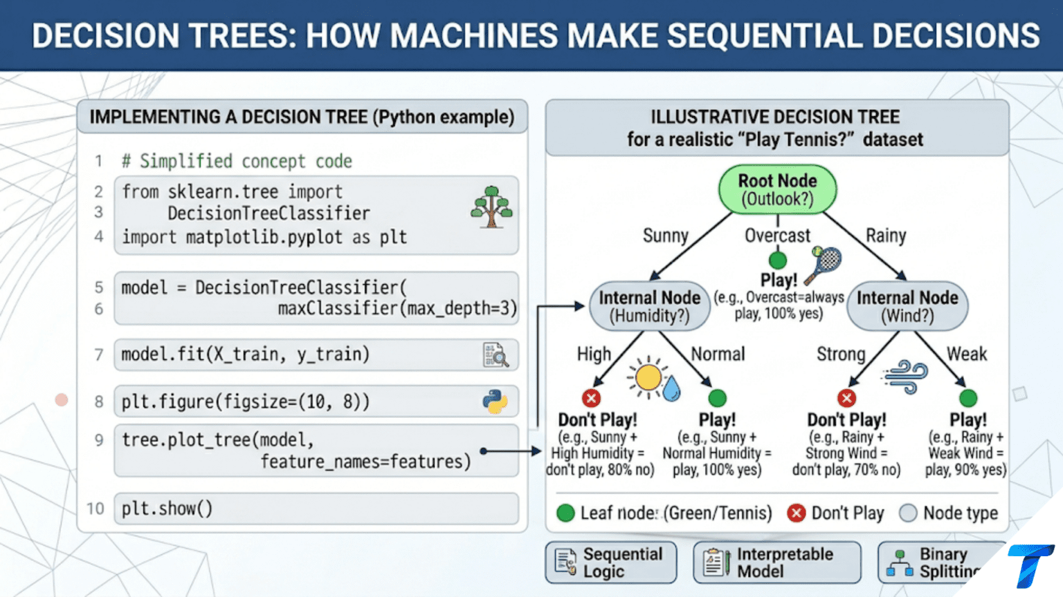
A decision tree is a supervised learning algorithm that makes predictions by asking a sequence of yes/no questions about the input features. Starting from a root node, each internal node tests one feature against a threshold, routing the data left (if the condition is true) or right (if false). The path from root to a leaf node defines a rule, and the leaf’s label (or value) is the prediction. Decision trees are interpretable by design — any prediction can be traced back through the exact sequence of conditions that produced it.
Introduction
When a doctor decides whether a patient needs emergency surgery, they do not run a single formula. They ask a series of questions: Is the blood pressure dangerously low? If yes — is there internal bleeding? If yes — call surgery. If no — try medication first. This sequential, rule-based reasoning is exactly what a decision tree formalizes mathematically.
Decision trees translate data into a flowchart of decisions. Each branch in the tree represents a test on a feature; each leaf represents a prediction. The elegance of this approach is that it mirrors the way humans naturally explain decisions — as a series of logical conditions — making decision trees among the most interpretable machine learning algorithms available.
Beyond interpretability, decision trees are the foundation of several of the most powerful algorithms in practical machine learning: Random Forests (Article 77), Gradient Boosting (Articles 81–83), and XGBoost (Articles 86–87) all build ensembles of decision trees. Understanding how individual trees work is therefore prerequisite knowledge for understanding the ensemble methods that dominate tabular data competitions.
This article builds a complete understanding of decision trees: the core structure, how trees are grown using splitting criteria, how depth and pruning control overfitting, implementation with scikit-learn, visualization, strengths and limitations, and the path from a single tree to understanding why ensembles are necessary.
Anatomy of a Decision Tree
Every decision tree consists of three types of nodes:
Root node: The topmost node, representing the entire dataset. The root’s splitting condition is the single most informative question that can be asked about the data.
Internal nodes (decision nodes): Each internal node tests one feature against a threshold (for numerical features: “Is feature X ≤ 4.5?”) or membership in a set (for categorical features: “Is color ∈ {red, blue}?”). Based on this test, data is routed to the left child (condition true) or right child (condition false).
Leaf nodes (terminal nodes): Nodes with no children. Each leaf stores a prediction: the majority class label (for classification) or the mean target value (for regression). When a new data point reaches a leaf, that leaf’s stored value is the prediction.
A Concrete Example
Consider classifying whether a mushroom is poisonous based on two features: cap color and odor. The tree might look like:
Is odor == "none"?
├─ YES → Is cap color == "red"?
│         ├─ YES → POISONOUS (leaf)
│         └─ NO  → EDIBLE (leaf)
└─ NO  → Is odor == "foul"?
          ├─ YES → POISONOUS (leaf)
└─ NO → EDIBLE (leaf)Each path from root to leaf is a classification rule. The rule “if odor is not none AND odor is foul → poisonous” is directly readable from the tree structure. This is what makes decision trees so valuable for domains requiring explanation: credit decisions, medical diagnoses, fraud detection, legal risk assessment.
How Trees Are Built: The Splitting Algorithm
The key question in decision tree construction is: at each node, which feature and threshold should be used to split the data? The answer comes from a splitting criterion — a measure of how much a split improves the purity of the resulting subsets.
The Greedy, Top-Down Approach
Decision trees are built using a greedy top-down approach called recursive binary splitting:
- Start with all training data at the root
- Search over all features and all possible thresholds for the split that maximizes the improvement in purity
- Split the data into left and right subsets using the best split
- Recursively apply steps 2–3 to each subset
- Stop when a stopping criterion is met (maximum depth, minimum samples, pure leaves)
This greedy approach does not guarantee the globally optimal tree — finding that would require evaluating all possible trees, which is NP-complete. Instead, it finds the locally best split at each node, which in practice produces trees that generalize well.
Measuring Impurity: Gini and Entropy
Two splitting criteria dominate decision tree implementations:
Gini Impurity measures how often a randomly chosen element from a set would be incorrectly labeled if it were randomly labeled according to the distribution in the subset:
where p_c is the proportion of class c in set S. A pure set (all one class) has Gini = 0. A maximally mixed binary set (50/50) has Gini = 0.5.
Entropy from information theory measures the average surprise (information content) of the class distribution:
A pure set has entropy = 0. A maximally mixed binary set has entropy = 1 bit.
Information Gain is the reduction in entropy (or Gini) achieved by a split:
The best split is the one that maximizes information gain — the greatest reduction in impurity when we divide S into left (S_L) and right (S_R) subsets.
import numpy as np
import matplotlib.pyplot as plt

def gini_impurity(class_counts):
    """
    Compute Gini impurity from class counts.

    Args:
        class_counts: Array or list of counts per class

    Returns:
        Gini impurity in [0, 0.5] for binary, [0, 1-1/C] for C classes
    """
    counts = np.array(class_counts, dtype=float)
    total  = counts.sum()
    if total == 0:
        return 0.0
    probs = counts / total
    return 1.0 - np.sum(probs ** 2)


def entropy(class_counts):
    """
    Compute entropy (bits) from class counts.

    Args:
        class_counts: Array or list of counts per class

    Returns:
        Entropy in [0, log2(C)] bits
    """
    counts = np.array(class_counts, dtype=float)
    total  = counts.sum()
    if total == 0:
        return 0.0
    probs  = counts / total
    # Avoid log(0): 0 * log(0) = 0 by convention
    log_probs = np.where(probs > 0, np.log2(probs), 0)
    return -np.sum(probs * log_probs)


def information_gain(parent_counts, left_counts, right_counts, criterion='entropy'):
    """
    Compute information gain of a binary split.

    Args:
        parent_counts: Class counts in parent node
        left_counts:   Class counts in left child
        right_counts:  Class counts in right child
        criterion:     'entropy' or 'gini'

    Returns:
        Information gain (reduction in impurity)
    """
    impurity_fn = entropy if criterion == 'entropy' else gini_impurity

    n_parent = sum(parent_counts)
    n_left   = sum(left_counts)
    n_right  = sum(right_counts)

    parent_impurity = impurity_fn(parent_counts)
    weighted_child  = (n_left  / n_parent) * impurity_fn(left_counts) + \
                      (n_right / n_parent) * impurity_fn(right_counts)

    return parent_impurity - weighted_child


# Demonstrate impurity measures
print("=== Impurity Measures: Examples ===\n")

scenarios = [
    ([100, 0],   "Pure class 0 (100, 0)"),
    ([50, 50],   "Perfectly balanced (50, 50)"),
    ([70, 30],   "70/30 split"),
    ([90, 10],   "90/10 split"),
    ([33, 33, 33], "Three-class balanced (33,33,33)"),
]

print(f"  {'Scenario':<35} | {'Gini':>7} | {'Entropy':>9}")
print("  " + "-" * 57)
for counts, label in scenarios:
    g = gini_impurity(counts)
    h = entropy(counts)
    print(f"  {label:<35} | {g:>7.4f} | {h:>9.4f}")

# Show information gain for different splits
print("\n=== Information Gain Examples ===\n")
print("  Parent: 100 samples, 50 class 0, 50 class 1\n")

split_scenarios = [
    ([40, 10], [10, 40], "Good split: separates classes"),
    ([30, 20], [20, 30], "Weak split: slight improvement"),
    ([25, 25], [25, 25], "Useless split: no improvement"),
    ([50, 0],  [0, 50],  "Perfect split: completely separates"),
]

parent = [50, 50]
for left, right, label in split_scenarios:
    ig_entropy = information_gain(parent, left, right, 'entropy')
    ig_gini    = information_gain(parent, left, right, 'gini')
    print(f"  {label}:")
    print(f"    Left={left}, Right={right}")
    print(f"    IG (entropy): {ig_entropy:.4f} | IG (gini): {ig_gini:.4f}")
    print()

# Visualize impurity as a function of class proportion (binary case)
fig, axes = plt.subplots(1, 2, figsize=(13, 5))

p_values = np.linspace(0, 1, 200)
gini_values   = [gini_impurity([p, 1-p]) for p in p_values]
entropy_values = [entropy([p, 1-p]) for p in p_values]

axes[0].plot(p_values, gini_values, 'coral', lw=2.5, label='Gini Impurity')
axes[0].plot(p_values, entropy_values, 'steelblue', lw=2.5, label='Entropy / 2')
# Scale entropy to [0, 0.5] for comparison
entropy_scaled = [e / 2 for e in entropy_values]
axes[0].plot(p_values, entropy_scaled, 'steelblue', lw=1.5,
             linestyle='--', label='Entropy (scaled to [0, 0.5])')
axes[0].set_xlabel('Proportion of Positive Class (p)', fontsize=12)
axes[0].set_ylabel('Impurity', fontsize=12)
axes[0].set_title('Gini vs Entropy: Binary Classification\n'
                   '(Both peak at p=0.5, reach 0 at pure nodes)',
                   fontsize=12, fontweight='bold')
axes[0].legend(fontsize=10)
axes[0].grid(True, alpha=0.3)

# Information gain surface for different split compositions
n = 100
ig_grid = np.zeros((50, 50))
splits_left  = np.linspace(1, 99, 50).astype(int)
splits_right = n - splits_left

for i, nl in enumerate(splits_left):
    for j, p_left in enumerate(np.linspace(0, 1, 50)):
        nr = n - nl
        n_pos_left  = int(nl * p_left)
        n_pos_right = max(0, 50 - n_pos_left)
        n_pos_right = min(n_pos_right, nr)
        ig_grid[i, j] = information_gain(
            [50, 50],
            [n_pos_left, nl - n_pos_left],
            [n_pos_right, nr - n_pos_right],
            'entropy'
        )

im = axes[1].imshow(ig_grid, aspect='auto', origin='lower',
                     cmap='YlOrRd', vmin=0, vmax=1)
plt.colorbar(im, ax=axes[1], label='Information Gain')
axes[1].set_xlabel('Fraction Positive in Left Child', fontsize=11)
axes[1].set_ylabel('Fraction of Data in Left Child', fontsize=11)
axes[1].set_title('Information Gain Landscape\n'
                   '(Red = good split, Yellow = poor split)',
                   fontsize=12, fontweight='bold')
axes[1].set_xticks([0, 25, 49])
axes[1].set_xticklabels(['0%', '50%', '100%'])
axes[1].set_yticks([0, 25, 49])
axes[1].set_yticklabels(['1%', '50%', '99%'])

plt.tight_layout()
plt.savefig('impurity_measures.png', dpi=150, bbox_inches='tight')
plt.show()
print("Saved: impurity_measures.png")Building a Decision Tree from Scratch
Implementing a decision tree reveals every design decision the algorithm makes. The core loop — find the best split, partition data, recurse — is surprisingly compact.
import numpy as np
from collections import Counter

class DecisionNode:
    """Represents one node in a decision tree."""
    __slots__ = ['feature', 'threshold', 'left', 'right',
                 'value', 'impurity', 'n_samples', 'class_counts']

    def __init__(self):
        # For internal (split) nodes
        self.feature   = None    # Feature index used for splitting
        self.threshold = None    # Threshold value for split
        self.left      = None    # Left child node (condition True)
        self.right     = None    # Right child node (condition False)
        # For leaf nodes
        self.value       = None  # Prediction (majority class or mean)
        # Metadata (stored for interpretability)
        self.impurity    = 0.0
        self.n_samples   = 0
        self.class_counts = None


class DecisionTreeClassifier:
    """
    Decision tree classifier built from scratch.

    Features:
    - Binary recursive splitting with Gini or Entropy criterion
    - max_depth, min_samples_split, min_samples_leaf stopping criteria
    - Majority-class prediction at leaves
    - predict_proba() using leaf class proportions
    - Human-readable tree printing
    """

    def __init__(self, criterion='gini', max_depth=None,
                 min_samples_split=2, min_samples_leaf=1,
                 random_state=None):
        """
        Args:
            criterion:          'gini' or 'entropy'
            max_depth:          Maximum tree depth (None = unlimited)
            min_samples_split:  Minimum samples to attempt a split
            min_samples_leaf:   Minimum samples allowed in each leaf
            random_state:       Seed for reproducibility (tie-breaking)
        """
        self.criterion         = criterion
        self.max_depth         = max_depth
        self.min_samples_split = min_samples_split
        self.min_samples_leaf  = min_samples_leaf
        self.random_state      = random_state
        self.root_             = None
        self.n_features_       = None
        self.classes_          = None
        self.feature_importances_ = None

    def _impurity(self, y):
        """Compute impurity of a label array."""
        if len(y) == 0:
            return 0.0
        counts = np.bincount(y, minlength=len(self.classes_))
        probs  = counts / len(y)
        if self.criterion == 'gini':
            return 1.0 - np.sum(probs ** 2)
        else:  # entropy
            log_probs = np.where(probs > 0, np.log2(probs + 1e-10), 0)
            return -np.sum(probs * log_probs)

    def _best_split(self, X, y):
        """
        Find the best feature and threshold to split (X, y).

        Searches all features and all mid-point thresholds between
        adjacent sorted values.

        Returns:
            best_feature, best_threshold, best_gain
            (Returns None, None, 0 if no beneficial split exists)
        """
        n, n_feat  = X.shape
        parent_imp = self._impurity(y)
        best_gain  = 0.0
        best_feat  = None
        best_thresh = None

        for feat in range(n_feat):
            # Get sorted unique values for this feature
            values   = np.sort(np.unique(X[:, feat]))

            # Try midpoints between consecutive unique values as thresholds
            if len(values) < 2:
                continue
            thresholds = (values[:-1] + values[1:]) / 2

            for thresh in thresholds:
                left_mask  = X[:, feat] <= thresh
                right_mask = ~left_mask

                n_left  = left_mask.sum()
                n_right = right_mask.sum()

                # Enforce min_samples_leaf constraint
                if n_left < self.min_samples_leaf or n_right < self.min_samples_leaf:
                    continue

                # Compute weighted impurity of children
                imp_left  = self._impurity(y[left_mask])
                imp_right = self._impurity(y[right_mask])

                gain = parent_imp - (n_left / n) * imp_left - (n_right / n) * imp_right

                if gain > best_gain:
                    best_gain   = gain
                    best_feat   = feat
                    best_thresh = thresh

        return best_feat, best_thresh, best_gain

    def _build(self, X, y, depth):
        """Recursively build the tree."""
        node = DecisionNode()
        node.n_samples    = len(y)
        node.impurity     = self._impurity(y)
        node.class_counts = np.bincount(y, minlength=len(self.classes_))

        # Majority class prediction for this node
        node.value = self.classes_[np.argmax(node.class_counts)]

        # Stopping criteria
        pure_node  = (len(np.unique(y)) == 1)
        max_depth_reached = (self.max_depth is not None and
                             depth >= self.max_depth)
        too_small  = (len(y) < self.min_samples_split)

        if pure_node or max_depth_reached or too_small:
            return node  # Leaf node

        # Find best split
        feat, thresh, gain = self._best_split(X, y)

        if feat is None or gain <= 0:
            return node  # No beneficial split found — make a leaf

        # Split data
        node.feature   = feat
        node.threshold = thresh
        left_mask  = X[:, feat] <= thresh
        right_mask = ~left_mask

        # Recurse on children
        node.left  = self._build(X[left_mask],  y[left_mask],  depth + 1)
        node.right = self._build(X[right_mask], y[right_mask], depth + 1)

        # Accumulate feature importances (weighted impurity reduction)
        self.feature_importances_[feat] += (
            (node.n_samples / self._n_samples_root) * gain
        )

        return node

    def fit(self, X, y):
        """Train the decision tree."""
        X = np.array(X, dtype=float)
        y = np.array(y)

        self.classes_          = np.unique(y)
        self.n_features_       = X.shape[1]
        self.feature_importances_ = np.zeros(self.n_features_)
        self._n_samples_root   = len(y)

        # Map labels to integers for bincount
        self._label_map = {c: i for i, c in enumerate(self.classes_)}
        y_int = np.array([self._label_map[label] for label in y])

        self.root_ = self._build(X, y_int, depth=0)

        # Normalize importances to sum to 1
        total = self.feature_importances_.sum()
        if total > 0:
            self.feature_importances_ /= total

        return self

    def _traverse(self, node, x):
        """Traverse the tree for a single sample."""
        if node.left is None and node.right is None:
            return node  # Leaf
        if x[node.feature] <= node.threshold:
            return self._traverse(node.left, x)
        else:
            return self._traverse(node.right, x)

    def predict(self, X):
        """Predict class labels."""
        X = np.array(X, dtype=float)
        predictions = []
        for x in X:
            leaf = self._traverse(self.root_, x)
            predictions.append(leaf.value)
        return np.array(predictions)

    def predict_proba(self, X):
        """Predict class probabilities from leaf class proportions."""
        X = np.array(X, dtype=float)
        probas = []
        for x in X:
            leaf  = self._traverse(self.root_, x)
            total = leaf.class_counts.sum()
            proba = leaf.class_counts / total if total > 0 else np.ones(len(self.classes_)) / len(self.classes_)
            probas.append(proba)
        return np.array(probas)

    def score(self, X, y):
        """Accuracy score."""
        return np.mean(self.predict(X) == np.array(y))

    def print_tree(self, node=None, depth=0, feature_names=None, max_depth=5):
        """Print a text representation of the tree."""
        if node is None:
            node = self.root_
        if depth > max_depth:
            print("  " * depth + "... (truncated)")
            return

        indent = "  " * depth
        is_leaf = (node.left is None and node.right is None)

        counts_str = ", ".join(f"cls{i}:{c}" for i, c in enumerate(node.class_counts))

        if is_leaf:
            print(f"{indent}[LEAF] Predict: {node.value} "
                  f"({counts_str}) n={node.n_samples}")
        else:
            feat_name = (feature_names[node.feature]
                         if feature_names else f"Feature[{node.feature}]")
            print(f"{indent}[Node] {feat_name} <= {node.threshold:.3f} "
                  f"(imp={node.impurity:.3f}, n={node.n_samples})")
            print(f"{indent}├─ True:")
            self.print_tree(node.left,  depth + 1, feature_names, max_depth)
            print(f"{indent}└─ False:")
            self.print_tree(node.right, depth + 1, feature_names, max_depth)


# Test our implementation vs scikit-learn
from sklearn.datasets import load_iris, load_wine
from sklearn.model_selection import train_test_split
from sklearn.tree import DecisionTreeClassifier as SklearnDT
from sklearn.preprocessing import LabelEncoder
import numpy as np

iris = load_iris()
X_ir, y_ir = iris.data, iris.target

X_tr_ir, X_te_ir, y_tr_ir, y_te_ir = train_test_split(
    X_ir, y_ir, test_size=0.25, random_state=42, stratify=y_ir
)

print("=== Decision Tree: From Scratch vs Scikit-learn ===\n")

for max_depth in [2, 3, 5, None]:
    # Our implementation
    our_dt = DecisionTreeClassifier(criterion='gini', max_depth=max_depth)
    our_dt.fit(X_tr_ir, y_tr_ir)
    our_acc = our_dt.score(X_te_ir, y_te_ir)

    # Scikit-learn reference
    sk_dt = SklearnDT(criterion='gini', max_depth=max_depth, random_state=42)
    sk_dt.fit(X_tr_ir, y_tr_ir)
    sk_acc = sk_dt.score(X_te_ir, y_te_ir)

    match = "~" if abs(our_acc - sk_acc) < 0.02 else "✗"
    print(f"  max_depth={str(max_depth):<5}: Our={our_acc:.4f}  Sklearn={sk_acc:.4f}  {match}")

print("\n=== Tree Structure (max_depth=3, Iris) ===\n")
our_dt3 = DecisionTreeClassifier(criterion='gini', max_depth=3)
our_dt3.fit(X_tr_ir, y_tr_ir)
our_dt3.print_tree(feature_names=iris.feature_names, max_depth=3)Controlling Tree Complexity: Depth, Pruning, and Stopping Criteria
An unconstrained decision tree will grow until every leaf is pure — perfectly memorizing the training data. This is extreme overfitting. Controlling complexity is therefore central to making decision trees generalize well.
Maximum Depth
The most direct control is max_depth: the tree cannot ask more than max_depth questions along any root-to-leaf path. Shallow trees (depth 2–4) have high bias but low variance and are robust; deep trees capture more patterns but risk overfitting.
Minimum Samples per Node
min_samples_split and min_samples_leaf stop growth when subsets become too small to support reliable estimates. A leaf with only 2 samples could have any class distribution by chance — requiring at least 10 or 20 samples per leaf forces the tree to generalize from larger, more reliable groups.
Minimum Impurity Decrease
min_impurity_decrease requires each split to produce at least a specified reduction in impurity. Splits that improve purity by only 0.0001% are likely fitting noise; requiring a minimum improvement threshold eliminates these.
Cost-Complexity Pruning
Scikit-learn’s ccp_alpha parameter implements cost-complexity pruning (also called weakest link pruning): after growing the full tree, it removes the subtrees that provide the least gain per unit complexity, with ccp_alpha controlling how aggressively to prune.
import numpy as np
import matplotlib.pyplot as plt
from sklearn.tree import DecisionTreeClassifier
from sklearn.datasets import make_classification
from sklearn.model_selection import train_test_split, cross_val_score

np.random.seed(42)
X_cmp, y_cmp = make_classification(
    n_samples=500, n_features=10, n_informative=6,
    n_redundant=2, random_state=42
)
X_tr_c, X_te_c, y_tr_c, y_te_c = train_test_split(
    X_cmp, y_cmp, test_size=0.25, random_state=42
)

# Effect of max_depth on train and test accuracy
print("=== max_depth vs Train/Test Accuracy ===\n")
print(f"  {'max_depth':>10} | {'n_leaves':>9} | {'Train Acc':>10} | {'Test Acc':>9} | {'Gap':>6}")
print("  " + "-" * 52)

train_accs = []
test_accs  = []
depths     = list(range(1, 20)) + [None]

for d in depths:
    dt = DecisionTreeClassifier(criterion='gini', max_depth=d, random_state=42)
    dt.fit(X_tr_c, y_tr_c)
    tr_acc = dt.score(X_tr_c, y_tr_c)
    te_acc = dt.score(X_te_c, y_te_c)
    train_accs.append(tr_acc)
    test_accs.append(te_acc)
    n_leaves = dt.get_n_leaves()
    d_label  = str(d) if d is not None else "None"
    print(f"  {d_label:>10} | {n_leaves:>9} | {tr_acc:>10.4f} | {te_acc:>9.4f} | "
          f"{tr_acc - te_acc:>6.4f}")

# Plot
fig, ax = plt.subplots(figsize=(11, 6))
depth_labels = list(range(1, 20)) + [20]  # Use 20 as "None" label for x-axis
ax.plot(depth_labels, train_accs, 'o-', color='steelblue', lw=2.5,
        markersize=7, label='Training Accuracy')
ax.plot(depth_labels, test_accs, 's-', color='coral', lw=2.5,
        markersize=7, label='Test Accuracy')
ax.fill_between(depth_labels,
                [t - v for t, v in zip(train_accs, test_accs)],
                0, alpha=0.1, color='red', label='Overfit gap')
ax.axvline(x=depth_labels[test_accs.index(max(test_accs))],
           color='green', linestyle='--', lw=2,
           label=f'Best test depth ≈ {depth_labels[test_accs.index(max(test_accs))]}')
ax.set_xlabel('Max Depth (20 = unconstrained)', fontsize=12)
ax.set_ylabel('Accuracy', fontsize=12)
ax.set_title('Decision Tree: max_depth vs Train/Test Accuracy\n'
             '(Depth beyond optimal increases overfitting without improving generalization)',
             fontsize=12, fontweight='bold')
ax.legend(fontsize=10)
ax.grid(True, alpha=0.3)
plt.tight_layout()
plt.savefig('dt_depth_vs_accuracy.png', dpi=150)
plt.show()
print("\nSaved: dt_depth_vs_accuracy.png")

# Cost-complexity pruning
print("\n=== Cost-Complexity Pruning (ccp_alpha) ===\n")
full_dt = DecisionTreeClassifier(random_state=42)
full_dt.fit(X_tr_c, y_tr_c)

# Get pruning path: sequence of alpha values that prune successively more
pruning_path = full_dt.cost_complexity_pruning_path(X_tr_c, y_tr_c)
ccp_alphas   = pruning_path.ccp_alphas[:-1]  # Drop last (trivially prunes all)

train_scores_ccp = []
test_scores_ccp  = []
n_nodes_ccp      = []

for alpha in ccp_alphas:
    dt_pruned = DecisionTreeClassifier(ccp_alpha=alpha, random_state=42)
    dt_pruned.fit(X_tr_c, y_tr_c)
    train_scores_ccp.append(dt_pruned.score(X_tr_c, y_tr_c))
    test_scores_ccp.append(dt_pruned.score(X_te_c, y_te_c))
    n_nodes_ccp.append(dt_pruned.tree_.node_count)

best_ccp_idx   = np.argmax(test_scores_ccp)
best_ccp_alpha = ccp_alphas[best_ccp_idx]

fig, axes = plt.subplots(1, 2, figsize=(14, 5))
axes[0].plot(ccp_alphas, train_scores_ccp, 'o-', color='steelblue', lw=2,
             markersize=5, label='Train')
axes[0].plot(ccp_alphas, test_scores_ccp, 's-', color='coral', lw=2,
             markersize=5, label='Test')
axes[0].axvline(x=best_ccp_alpha, color='green', linestyle='--', lw=2,
                label=f'Best α={best_ccp_alpha:.4f}')
axes[0].set_xlabel('ccp_alpha (pruning strength)', fontsize=11)
axes[0].set_ylabel('Accuracy', fontsize=11)
axes[0].set_title('Accuracy vs Pruning Strength', fontsize=11, fontweight='bold')
axes[0].legend(fontsize=9)
axes[0].grid(True, alpha=0.3)

axes[1].plot(ccp_alphas, n_nodes_ccp, 'o-', color='mediumpurple', lw=2, markersize=5)
axes[1].axvline(x=best_ccp_alpha, color='green', linestyle='--', lw=2)
axes[1].set_xlabel('ccp_alpha (pruning strength)', fontsize=11)
axes[1].set_ylabel('Number of Nodes', fontsize=11)
axes[1].set_title('Tree Size vs Pruning Strength\n(Higher α = simpler tree)',
                   fontsize=11, fontweight='bold')
axes[1].grid(True, alpha=0.3)

plt.suptitle('Cost-Complexity Pruning: ccp_alpha Sweep', fontsize=13,
             fontweight='bold')
plt.tight_layout()
plt.savefig('dt_ccp_pruning.png', dpi=150)
plt.show()
print("Saved: dt_ccp_pruning.png")Visualizing Decision Trees
One of decision trees’ greatest strengths is direct visualization. A tree with moderate depth can be plotted and immediately understood by non-technical stakeholders.
from sklearn.tree import DecisionTreeClassifier, plot_tree, export_text
from sklearn.datasets import load_iris, load_breast_cancer
from sklearn.model_selection import train_test_split
from sklearn.preprocessing import StandardScaler
import matplotlib.pyplot as plt
import numpy as np

# Train on Iris — a classic, highly interpretable dataset
iris = load_iris()
X_ir_v, y_ir_v = iris.data, iris.target
X_tr_v, X_te_v, y_tr_v, y_te_v = train_test_split(
    X_ir_v, y_ir_v, test_size=0.25, random_state=42, stratify=y_ir_v
)

dt_vis = DecisionTreeClassifier(max_depth=3, criterion='gini', random_state=42)
dt_vis.fit(X_tr_v, y_tr_v)

print(f"Tree accuracy: {dt_vis.score(X_te_v, y_te_v):.4f}")
print(f"Depth: {dt_vis.get_depth()} | Leaves: {dt_vis.get_n_leaves()}\n")

# Text representation
print("=== Text Tree ===\n")
print(export_text(dt_vis, feature_names=iris.feature_names))

# Visual plot
fig, ax = plt.subplots(figsize=(16, 8))
plot_tree(
    dt_vis,
    feature_names=iris.feature_names,
    class_names=iris.target_names,
    filled=True,           # Color nodes by majority class
    rounded=True,          # Rounded boxes
    impurity=True,         # Show Gini impurity
    precision=3,           # Decimal places for thresholds
    ax=ax,
    fontsize=11
)
ax.set_title('Decision Tree: Iris Dataset (max_depth=3)\n'
             'Color intensity = class purity at each node',
             fontsize=14, fontweight='bold')
plt.tight_layout()
plt.savefig('decision_tree_iris_visual.png', dpi=150, bbox_inches='tight')
plt.show()
print("Saved: decision_tree_iris_visual.png")

# Decision boundary visualization (2D)
def plot_decision_tree_boundary(X, y, dt, feature_names, class_names, title):
    """Visualize decision tree boundary in 2D feature space."""
    x_min, x_max = X[:, 0].min() - 0.5, X[:, 0].max() + 0.5
    y_min, y_max = X[:, 1].min() - 0.5, X[:, 1].max() + 0.5

    xx, yy = np.meshgrid(np.linspace(x_min, x_max, 300),
                          np.linspace(y_min, y_max, 300))
    Z = dt.predict(np.c_[xx.ravel(), yy.ravel()]).reshape(xx.shape)

    colors_bg  = ['#d0e8f8', '#f8d0d0', '#d0f8d0']
    colors_pts = ['steelblue', 'coral', 'mediumseagreen']

    fig, ax = plt.subplots(figsize=(9, 7))
    ax.contourf(xx, yy, Z, alpha=0.35,
                colors=colors_bg[:len(np.unique(y))])
    ax.contour(xx, yy, Z, colors='black', linewidths=0.8, alpha=0.5)

    for cls, color in zip(np.unique(y), colors_pts):
        mask = y == cls
        ax.scatter(X[mask, 0], X[mask, 1], c=color, edgecolors='white',
                   s=50, linewidth=0.5, label=class_names[cls], alpha=0.85)

    ax.set_xlabel(feature_names[0], fontsize=11)
    ax.set_ylabel(feature_names[1], fontsize=11)
    ax.set_title(title, fontsize=12, fontweight='bold')
    ax.legend(fontsize=10)
    ax.grid(True, alpha=0.2)
    plt.tight_layout()
    plt.savefig('dt_decision_boundary.png', dpi=150)
    plt.show()
    print("Saved: dt_decision_boundary.png")


# Use petal features only (2D visualization)
X_2d = X_ir_v[:, 2:]  # petal length, petal width
dt_2d = DecisionTreeClassifier(max_depth=4, criterion='gini', random_state=42)
dt_2d.fit(X_2d, y_ir_v)

plot_decision_tree_boundary(
    X_2d, y_ir_v, dt_2d,
    feature_names=['Petal Length (cm)', 'Petal Width (cm)'],
    class_names=iris.target_names,
    title='Decision Tree Boundary: Iris (Petal Features, max_depth=4)\n'
          'Axis-aligned splits create rectangular decision regions'
)Feature Importance in Decision Trees
Each time a feature is used for a split, it contributes to the tree’s predictive power. Decision trees track this by summing the weighted impurity reduction across all nodes where the feature was used:
These importances are normalized to sum to 1, providing a ranking of feature relevance.
from sklearn.tree import DecisionTreeClassifier
from sklearn.datasets import load_breast_cancer
from sklearn.model_selection import train_test_split
import numpy as np
import matplotlib.pyplot as plt

cancer = load_breast_cancer()
X_ca, y_ca = cancer.data, cancer.target

X_tr_ca, X_te_ca, y_tr_ca, y_te_ca = train_test_split(
    X_ca, y_ca, test_size=0.25, random_state=42, stratify=y_ca
)

dt_ca = DecisionTreeClassifier(max_depth=5, criterion='gini', random_state=42)
dt_ca.fit(X_tr_ca, y_tr_ca)

importances = dt_ca.feature_importances_
feature_names = cancer.feature_names

sorted_idx = np.argsort(importances)[::-1]
top_n = 15

fig, ax = plt.subplots(figsize=(11, 6))
bars = ax.bar(range(top_n),
              importances[sorted_idx[:top_n]],
              color='steelblue', edgecolor='white', linewidth=0.5)
ax.set_xticks(range(top_n))
ax.set_xticklabels([feature_names[i] for i in sorted_idx[:top_n]],
                    rotation=45, ha='right', fontsize=9)
ax.set_ylabel('Feature Importance (mean impurity decrease)', fontsize=11)
ax.set_title('Decision Tree Feature Importances: Breast Cancer Dataset\n'
             '(Normalized sum = 1.0)', fontsize=12, fontweight='bold')
ax.grid(True, alpha=0.3, axis='y')
plt.tight_layout()
plt.savefig('dt_feature_importances.png', dpi=150)
plt.show()

print("=== Top 10 Feature Importances ===\n")
for rank, idx in enumerate(sorted_idx[:10], 1):
    print(f"  {rank:2d}. {feature_names[idx]:<35}: {importances[idx]:.4f}")
Important caveat: Decision tree feature importances have a known bias toward features with many possible values (high cardinality), because those features offer more candidate thresholds and thus more opportunities to appear as the best split. For more unbiased importance estimates, use permutation importance or Random Forest importance averaged across many trees.
Strengths and Limitations
Strengths
Interpretability. A shallow tree (depth 3–5) can be printed, plotted, and explained to any stakeholder. The path from root to leaf is a human-readable rule. This is unmatched by any other competitive algorithm and makes decision trees the preferred choice in regulated domains where decisions must be justified.
No feature scaling required. Because trees make decisions based on thresholds (is feature X > 4.5?), the absolute scale of features is irrelevant. Standardization, normalization, or log-transformation have no effect on the tree structure.
Handles mixed feature types. Numerical and categorical features can coexist without encoding tricks (in implementations that support it). sklearn requires encoding, but the underlying algorithm accommodates categorical splits naturally.
Handles nonlinear relationships. Trees can capture arbitrarily complex decision boundaries — any region in feature space can be approximated by a deep enough tree. This is more flexible than linear models.
Naturally handles multi-class. No one-vs-rest wrapper needed. The splitting criterion already handles C-class problems.
Fast inference. Predicting a sample requires at most max_depth comparisons — O(log n) for a balanced tree. This is extremely fast at inference time.
Limitations
Overfitting. Without regularization, a tree will grow until every leaf contains exactly one sample. Deep trees memorize training data perfectly and generalize poorly. Controlling depth, minimum leaf size, and pruning is essential.
High variance. Decision trees are notoriously unstable: a small change to the training data can produce a completely different tree structure. This variance is the primary motivation for Random Forests, which average many trees to reduce variance.
Axis-aligned boundaries only. Each split tests one feature at a time, producing rectangular decision regions. Diagonal or circular boundaries require many splits to approximate. A linear boundary that cuts diagonally through the feature space will be very poorly approximated by a decision tree.
Biased toward high-cardinality features. As noted above, features with many values have more candidate thresholds and are more likely to appear as the best split, even if they are not actually more informative.
Poor performance on regression with extrapolation. Decision tree regressors predict the mean value in each leaf. This means they cannot extrapolate beyond the range of training values — predictions plateau at the training data boundary.
Decision Trees for Regression
Everything above applies to classification. Decision trees extend naturally to regression with two changes: the splitting criterion becomes variance reduction instead of Gini/entropy, and the leaf prediction becomes the mean target value of the leaf’s samples rather than the majority class.
Variance Reduction as a Splitting Criterion
For regression, impurity is measured by the variance of target values in a node:
The best split is the one that most reduces the weighted variance of the children relative to the parent:
At each leaf, the prediction is the mean of all training samples that reached that leaf. This produces a piecewise constant approximation to the true function — the predicted surface is a step function.
import numpy as np
import matplotlib.pyplot as plt
from sklearn.tree import DecisionTreeRegressor
from sklearn.datasets import fetch_california_housing
from sklearn.model_selection import train_test_split, cross_val_score
from sklearn.metrics import mean_squared_error, r2_score

# Synthetic example first: sinusoidal function
np.random.seed(42)
X_reg_1d = np.sort(np.random.uniform(0, 4 * np.pi, 300)).reshape(-1, 1)
y_reg_1d = np.sin(X_reg_1d.ravel()) + 0.5 * np.cos(2 * X_reg_1d.ravel()) + \
           np.random.normal(0, 0.2, 300)

# Test different depths
fig, axes = plt.subplots(2, 2, figsize=(14, 10))
x_plot = np.linspace(0, 4 * np.pi, 1000).reshape(-1, 1)
y_true = np.sin(x_plot.ravel()) + 0.5 * np.cos(2 * x_plot.ravel())

for ax, max_d in zip(axes.flatten(), [1, 3, 7, None]):
    dt_reg = DecisionTreeRegressor(max_depth=max_d, random_state=42)
    dt_reg.fit(X_reg_1d, y_reg_1d)
    y_pred = dt_reg.predict(x_plot)

    ax.scatter(X_reg_1d, y_reg_1d, color='steelblue', s=15, alpha=0.5,
               label='Training data')
    ax.plot(x_plot, y_true, 'k--', lw=1.5, alpha=0.6, label='True function')
    ax.plot(x_plot, y_pred, 'coral', lw=2.5,
            label=f'DT prediction (depth={max_d})')

    train_r2 = r2_score(y_reg_1d, dt_reg.predict(X_reg_1d))
    n_leaves = dt_reg.get_n_leaves()
    ax.set_title(f'max_depth = {max_d}  |  {n_leaves} leaves  |  Train R² = {train_r2:.3f}',
                 fontsize=11, fontweight='bold')
    ax.set_xlabel('X', fontsize=10)
    ax.set_ylabel('y', fontsize=10)
    ax.legend(fontsize=8, loc='upper right')
    ax.grid(True, alpha=0.3)

plt.suptitle('Decision Tree Regression: Piecewise Constant Approximation\n'
             '(Each leaf predicts the mean of its training samples)',
             fontsize=13, fontweight='bold', y=1.01)
plt.tight_layout()
plt.savefig('dt_regression_depth_comparison.png', dpi=150, bbox_inches='tight')
plt.show()
print("Saved: dt_regression_depth_comparison.png")

# Real dataset: California housing
housing = fetch_california_housing()
X_h, y_h = housing.data, housing.target

X_tr_h, X_te_h, y_tr_h, y_te_h = train_test_split(
    X_h, y_h, test_size=0.20, random_state=42
)

print("\n=== Decision Tree Regression: California Housing ===\n")
print(f"  {'max_depth':>10} | {'n_leaves':>9} | {'Train R²':>9} | {'Test R²':>8} | {'Test RMSE':>10}")
print("  " + "-" * 56)

for d in [2, 3, 5, 7, 10, 15, None]:
    dtr = DecisionTreeRegressor(max_depth=d, random_state=42)
    dtr.fit(X_tr_h, y_tr_h)

    tr_r2   = dtr.score(X_tr_h, y_tr_h)
    te_r2   = dtr.score(X_te_h, y_te_h)
    te_rmse = np.sqrt(mean_squared_error(y_te_h, dtr.predict(X_te_h)))
    n_leaves = dtr.get_n_leaves()
    d_label  = str(d) if d is not None else "None"

    print(f"  {d_label:>10} | {n_leaves:>9} | {tr_r2:>9.4f} | {te_r2:>8.4f} | {te_rmse:>10.4f}")

# Cross-validated depth selection
print("\n  Cross-validated depth selection:")
cv_results = []
depth_range = list(range(2, 16))
for d in depth_range:
    dtr_cv = DecisionTreeRegressor(max_depth=d, random_state=42)
    scores = cross_val_score(dtr_cv, X_h, y_h, cv=5, scoring='r2', n_jobs=-1)
    cv_results.append(scores.mean())

best_depth = depth_range[np.argmax(cv_results)]
print(f"  Best max_depth by 5-Fold CV: {best_depth} "
      f"(CV R² = {max(cv_results):.4f})")
print(f"\n  Note: For regression, decision trees are often outperformed by")
print(f"  gradient boosted trees due to their piecewise-constant limitation.")
print(f" The true function is smooth; DTs approximate it with steps.")The Extrapolation Limitation
A critical weakness specific to decision tree regression is its inability to extrapolate. Since each leaf predicts the mean of its training samples, and no training samples exist beyond the training range, the tree simply returns the extreme leaf’s mean for any out-of-range query. This means decision tree regressors should never be applied to data where extrapolation beyond the training range is required.
import numpy as np
import matplotlib.pyplot as plt
from sklearn.tree import DecisionTreeRegressor
from sklearn.linear_model import LinearRegression

# Show extrapolation failure
np.random.seed(42)
X_train_ext = np.linspace(0, 10, 100).reshape(-1, 1)
y_train_ext = 2 * X_train_ext.ravel() + np.random.normal(0, 1, 100)

# Test range extends beyond training range
X_test_ext = np.linspace(-2, 14, 300).reshape(-1, 1)
y_true_ext = 2 * X_test_ext.ravel()

dt_ext  = DecisionTreeRegressor(max_depth=5, random_state=42)
lr_ext  = LinearRegression()
dt_ext.fit(X_train_ext, y_train_ext)
lr_ext.fit(X_train_ext, y_train_ext)

fig, ax = plt.subplots(figsize=(11, 5))
ax.scatter(X_train_ext, y_train_ext, color='steelblue', s=20, alpha=0.6,
           label='Training data (X ∈ [0, 10])')
ax.plot(X_test_ext, y_true_ext, 'k--', lw=1.5, alpha=0.6, label='True function (y=2x)')
ax.plot(X_test_ext, dt_ext.predict(X_test_ext), 'coral', lw=2.5,
        label='Decision Tree (fails beyond training range)')
ax.plot(X_test_ext, lr_ext.predict(X_test_ext), 'mediumseagreen', lw=2.5,
        label='Linear Regression (extrapolates correctly)')

ax.axvspan(-2, 0, alpha=0.07, color='red', label='Extrapolation region')
ax.axvspan(10, 14, alpha=0.07, color='red')
ax.axvline(x=0, color='red', linestyle=':', lw=1.5, alpha=0.7)
ax.axvline(x=10, color='red', linestyle=':', lw=1.5, alpha=0.7)

ax.set_xlabel('X', fontsize=12)
ax.set_ylabel('y', fontsize=12)
ax.set_title('Decision Tree Regression: Extrapolation Failure\n'
             'Predictions plateau at training range boundaries',
             fontsize=12, fontweight='bold')
ax.legend(fontsize=9, loc='upper left')
ax.grid(True, alpha=0.3)
plt.tight_layout()
plt.savefig('dt_regression_extrapolation.png', dpi=150)
plt.show()
print("Saved: dt_regression_extrapolation.png")
print("\n  Key takeaway: Decision trees cannot extrapolate.")
print("  Use linear models or neural networks when predictions")
print("  outside the training range are required.")
Why Single Trees Lead to Ensembles
The single most important weakness of decision trees is their high variance. The same dataset, split differently, produces dramatically different trees:
import numpy as np
from sklearn.tree import DecisionTreeClassifier
from sklearn.datasets import make_classification
from sklearn.model_selection import train_test_split

np.random.seed(0)
X_var, y_var = make_classification(
    n_samples=500, n_features=10, n_informative=6, random_state=42
)

print("=== Decision Tree Variance Across Random Seeds ===\n")
print(f"  Same dataset, same max_depth=5, different train-test splits:\n")
print(f"  {'Seed':>6} | {'Train Acc':>10} | {'Test Acc':>9} | {'n_leaves':>9}")
print("  " + "-" * 42)

test_accs = []
for seed in range(20):
    X_tr_v2, X_te_v2, y_tr_v2, y_te_v2 = train_test_split(
        X_var, y_var, test_size=0.30, random_state=seed
    )
    dt_v = DecisionTreeClassifier(max_depth=5, random_state=42)
    dt_v.fit(X_tr_v2, y_tr_v2)
    tr_acc = dt_v.score(X_tr_v2, y_tr_v2)
    te_acc = dt_v.score(X_te_v2, y_te_v2)
    test_accs.append(te_acc)
    if seed < 10:
        print(f"  {seed:>6} | {tr_acc:>10.4f} | {te_acc:>9.4f} | {dt_v.get_n_leaves():>9}")

print(f"\n  Test accuracy statistics over 20 seeds:")
print(f"  Mean: {np.mean(test_accs):.4f}")
print(f"  Std:  {np.std(test_accs):.4f}")
print(f"  Min:  {np.min(test_accs):.4f}")
print(f"  Max:  {np.max(test_accs):.4f}")
print(f"\n  Range: {np.max(test_accs) - np.min(test_accs):.4f}")
print(f"\n  → This variance motivates Random Forests:")
print(f" Average 100 trees → much lower variance, similar bias.")This variance is the reason why Random Forests (Article 77) and other ensemble methods were developed. By training many trees on different subsets of data and averaging their predictions, the variance is dramatically reduced while bias remains similar. The single decision tree is therefore best understood as a building block for these more powerful ensembles — valuable alone for its interpretability, but typically superseded in predictive performance by ensemble variants.
Summary
Decision trees build predictions by asking a sequence of yes/no questions about features, routing each sample down a path from root to leaf. The questions are selected greedily to maximize purity improvement (measured by Gini impurity or entropy) at each step.
The fundamental tension in decision trees is the depth-accuracy tradeoff: deeper trees capture more patterns but overfit more severely. Controlling depth, minimum leaf sizes, and applying cost-complexity pruning brings trees from perfectly memorizing training data to genuinely generalizing.
Feature importances — summed weighted impurity reductions — provide a natural ranking of feature relevance, though with caveats about high-cardinality bias. The direct visualization of tree structure, where any prediction can be traced through a human-readable sequence of conditions, makes decision trees uniquely valuable for interpretable machine learning.
Their high variance — that instability to small changes in the training data — is both their primary weakness and the foundation for ensemble methods. Understanding how and why a single decision tree overfits, and how its variance is measured, directly motivates understanding why Random Forests average many trees, and why Gradient Boosting corrects residuals sequentially.