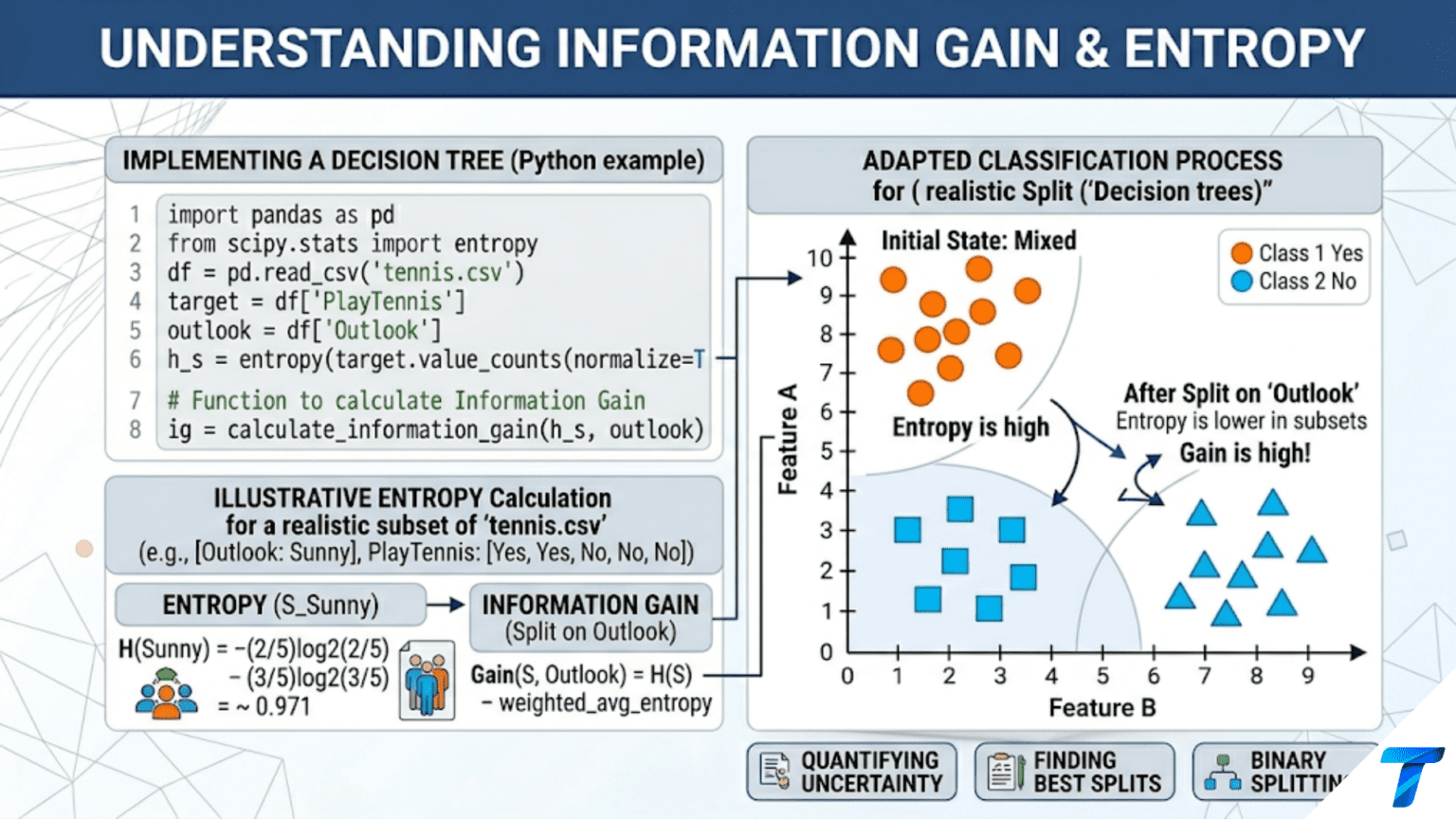
Entropy measures the uncertainty or impurity in a set of labels: a node where all samples belong to one class has entropy 0 (no uncertainty), while a node with equally distributed classes has maximum entropy. Information gain is the reduction in entropy achieved by splitting a node into two children — the best split is the one that reduces entropy the most. Decision trees use information gain to greedily select which feature and threshold to split on at each node.
Introduction
Claude Shannon, working at Bell Labs in 1948, published “A Mathematical Theory of Communication” — one of the most influential papers of the twentieth century. Shannon’s goal was to quantify how much information is contained in a message, enabling engineers to design efficient communication systems. His answer was entropy, a mathematical measure of uncertainty.
Decades later, machine learning researchers realized that Shannon’s entropy answered a question at the heart of decision tree construction: which question about the data reduces uncertainty the most? If you can measure uncertainty precisely, you can measure how much any given split reduces it — and that measurement, called information gain, is the criterion by which decision trees choose their splits.
Understanding entropy and information gain is therefore understanding the internal logic of decision trees at its deepest level. It also opens doors to related concepts that appear across machine learning: cross-entropy as a loss function for neural networks, mutual information for feature selection, KL divergence for comparing probability distributions, and the information-theoretic foundations of compression and generalization.
This article builds complete mathematical and intuitive understanding of entropy, information gain, and their extensions — from first principles through Python implementation to practical applications in feature selection and model evaluation.
Entropy: Measuring Uncertainty
The Intuition
Suppose you flip a fair coin. Before seeing the result, you are maximally uncertain — it could be heads or tails with equal probability. After seeing the result, your uncertainty is completely resolved. The coin flip conveys exactly 1 bit of information.
Now suppose the coin is extremely biased: 99% heads, 1% tails. Before you flip it, you are already quite certain it will be heads. You are surprised only 1% of the time. The average information conveyed per flip is much less than 1 bit — because most outcomes are predictable.
Shannon formalized this intuition: information is surprise. Rare events (p ≈ 0) carry a lot of information when they occur. Common events (p ≈ 1) carry little information — you already expected them.
The information content of observing a single outcome with probability p is:
When p = 1 (certain outcome), I(p) = 0 bits — no surprise. When p = 0.5, I(p) = 1 bit. When p = 0.01, I(p) ≈ 6.64 bits — very surprising.
Shannon Entropy: Expected Information
Entropy is the expected information content across all possible outcomes:
where p_c is the probability of class c and the sum runs over all C classes. Convention: 0 × log(0) = 0.
For binary classification with p the probability of the positive class:
This function has several key properties:
- H(0) = H(1) = 0: Pure sets (all one class) have zero entropy
- H(0.5) = 1 bit: A 50/50 split has maximum entropy for binary classification
- H is symmetric: H(p) = H(1-p)
- H is concave: mixing never reduces entropy
import numpy as np
import matplotlib.pyplot as plt
from matplotlib.gridspec import GridSpec

def entropy_binary(p):
    """
    Binary entropy function H(p) = -p*log2(p) - (1-p)*log2(1-p).

    Args:
        p: Probability of positive class (scalar or array)

    Returns:
        Entropy in bits
    """
    p = np.asarray(p, dtype=float)
    # Avoid log(0): use numerical safe version
    eps = 1e-12
    p_safe   = np.clip(p, eps, 1 - eps)
    q_safe   = 1 - p_safe
    return -p_safe * np.log2(p_safe) - q_safe * np.log2(q_safe)


def entropy_multiclass(class_counts):
    """
    Shannon entropy for an arbitrary number of classes.

    Args:
        class_counts: Array or list of counts per class

    Returns:
        Entropy in bits
    """
    counts = np.array(class_counts, dtype=float)
    total  = counts.sum()
    if total == 0:
        return 0.0
    probs = counts / total
    # Only include non-zero probabilities (0*log(0) = 0 by convention)
    nonzero = probs[probs > 0]
    return -np.sum(nonzero * np.log2(nonzero))


def information_content(p):
    """
    Surprisal (self-information) of a single outcome with probability p.

    Args:
        p: Probability of the outcome

    Returns:
        Information content in bits
    """
    if p <= 0:
        return float('inf')
    return -np.log2(p)


# Demonstrate the binary entropy function
print("=== Binary Entropy: Key Values ===\n")
print(f"  {'p (positive class %)':>25} | {'H(p) bits':>12} | Interpretation")
print("  " + "-" * 62)

test_probs = [0.0, 0.01, 0.1, 0.25, 0.5, 0.75, 0.9, 0.99, 1.0]
for p in test_probs:
    h = entropy_binary(p) if 0 < p < 1 else 0.0
    if p == 0.5:
        interp = "Maximum uncertainty (50/50 split)"
    elif p in (0.0, 1.0):
        interp = "Perfect certainty — pure node"
    elif p < 0.1 or p > 0.9:
        interp = "Near-pure — low uncertainty"
    else:
        interp = "Moderate uncertainty"
    print(f"  {p*100:>24.1f}% | {h:>12.6f} | {interp}")


# Demonstrate information content (surprisal)
print("\n=== Information Content (Surprisal) ===\n")
print(f"  {'Event probability':>20} | {'Bits of info':>14} | Example")
print("  " + "-" * 60)

events = [
    (0.5,    "Fair coin flip"),
    (1/6,    "Rolling a 6 on a die"),
    (0.1,    "10% probability event"),
    (0.01,   "Rare event (1%)"),
    (1/1024, "One specific card from ~1000"),
    (1e-6,   "Lottery win estimate"),
]

for p, example in events:
    bits = information_content(p)
    print(f"  {p:>20.6f} | {bits:>14.4f} | {example}")


# Multiclass entropy examples
print("\n=== Multiclass Entropy ===\n")
print(f"  {'Distribution':>35} | {'H (bits)':>10} | Notes")
print("  " + "-" * 68)

multiclass_examples = [
    ([100, 0, 0],    "Pure (all class 0)"),
    ([50, 50, 0],    "Two-class 50/50 (3 labels)"),
    ([34, 33, 33],   "Three-class near-uniform"),
    ([25, 25, 25, 25], "Four-class uniform"),
    ([90, 5, 5],     "Dominant class 0"),
    ([10, 45, 45],   "Two dominant classes"),
]

for counts, desc in multiclass_examples:
    h = entropy_multiclass(counts)
    max_h = np.log2(len(counts))  # Maximum possible for this many classes
    print(f"  {desc:>35} | {h:>10.4f} | max={max_h:.4f}")


# Full visualization of entropy functions
fig = plt.figure(figsize=(16, 12))
gs  = GridSpec(2, 2, figure=fig, hspace=0.4, wspace=0.35)

# 1. Binary entropy curve
ax1 = fig.add_subplot(gs[0, 0])
p_vals = np.linspace(0.001, 0.999, 500)
h_vals = entropy_binary(p_vals)
ax1.plot(p_vals, h_vals, 'steelblue', lw=2.5)
ax1.fill_between(p_vals, h_vals, alpha=0.15, color='steelblue')
ax1.axhline(y=1.0, color='coral', linestyle='--', lw=1.5, alpha=0.7,
            label='Maximum entropy = 1 bit')
ax1.axvline(x=0.5, color='coral', linestyle=':', lw=1.5, alpha=0.7)
# Annotate key points
for p_ann, h_ann, label in [(0.1, entropy_binary(0.1), '10/90\nsplit'),
                              (0.5, 1.0, '50/50\nsplit'),
                              (0.9, entropy_binary(0.9), '90/10\nsplit')]:
    ax1.annotate(f'{label}\nH={h_ann:.3f}',
                 xy=(p_ann, h_ann), xytext=(p_ann + 0.05, h_ann - 0.15),
                 fontsize=8, arrowprops=dict(arrowstyle='->', lw=0.8))
ax1.set_xlabel('p (fraction of positive class)', fontsize=11)
ax1.set_ylabel('H(p) in bits', fontsize=11)
ax1.set_title('Binary Entropy Function\nH(p) = −p log₂(p) − (1−p) log₂(1−p)',
              fontsize=11, fontweight='bold')
ax1.legend(fontsize=9)
ax1.grid(True, alpha=0.3)

# 2. Surprisal (information content) curve
ax2 = fig.add_subplot(gs[0, 1])
p_surp = np.linspace(0.001, 1.0, 500)
i_vals = -np.log2(p_surp)
ax2.plot(p_surp, i_vals, 'coral', lw=2.5)
ax2.fill_between(p_surp, i_vals, alpha=0.15, color='coral')
ax2.axhline(y=1.0, color='steelblue', linestyle='--', lw=1.5, alpha=0.7,
            label='1 bit (fair coin flip)')
ax2.set_xlabel('Event probability p', fontsize=11)
ax2.set_ylabel('Surprisal = −log₂(p) bits', fontsize=11)
ax2.set_title('Surprisal (Self-Information)\nRare events carry more information',
              fontsize=11, fontweight='bold')
ax2.set_ylim([0, 10])
ax2.legend(fontsize=9)
ax2.grid(True, alpha=0.3)

# 3. Entropy for 2, 3, 4 classes (uniform distribution as reference)
ax3 = fig.add_subplot(gs[1, 0])
n_classes_range = np.arange(2, 21)
max_entropies   = np.log2(n_classes_range)
ax3.plot(n_classes_range, max_entropies, 'o-', color='mediumseagreen',
         lw=2.5, markersize=8, label='Max entropy (uniform dist.)')
ax3.fill_between(n_classes_range, max_entropies, alpha=0.15,
                 color='mediumseagreen')
ax3.set_xlabel('Number of Classes C', fontsize=11)
ax3.set_ylabel('Maximum Entropy (bits)', fontsize=11)
ax3.set_title('Maximum Entropy Grows with Number of Classes\nH_max = log₂(C)',
              fontsize=11, fontweight='bold')
ax3.legend(fontsize=9)
ax3.grid(True, alpha=0.3)

# 4. Entropy for skewed distributions
ax4 = fig.add_subplot(gs[1, 1])
# Show entropy as function of majority class proportion for 3-class problem
# with remaining probability split evenly among others
majority_probs = np.linspace(1/3, 0.999, 200)
entropies_3cls = []
for p_maj in majority_probs:
    p_others = (1 - p_maj) / 2
    entropies_3cls.append(entropy_multiclass([p_maj, p_others, p_others]))
ax4.plot(majority_probs * 100, entropies_3cls, 'mediumpurple', lw=2.5)
ax4.axhline(y=np.log2(3), color='coral', linestyle='--', lw=1.5,
            label=f'Max entropy = log₂(3) ≈ {np.log2(3):.3f} bits')
ax4.axvline(x=100/3, color='gray', linestyle=':', lw=1.5, alpha=0.7,
            label='Uniform (33.3%)')
ax4.set_xlabel('Majority Class % (other two split evenly)', fontsize=11)
ax4.set_ylabel('Entropy (bits)', fontsize=11)
ax4.set_title('Three-Class Entropy vs Majority Class Dominance',
              fontsize=11, fontweight='bold')
ax4.legend(fontsize=9)
ax4.grid(True, alpha=0.3)

plt.suptitle('Shannon Entropy: The Foundation of Decision Tree Splitting',
             fontsize=14, fontweight='bold', y=1.01)
plt.savefig('entropy_fundamentals.png', dpi=150, bbox_inches='tight')
plt.show()
print("Saved: entropy_fundamentals.png")Information Gain: Measuring Split Quality
With entropy as a measure of impurity, we can now measure how much any proposed split reduces impurity. This is information gain:
where S is the dataset, A is the splitting attribute, and S_v is the subset with attribute value v. For binary splits (the only type used in most decision tree implementations):
The information gain is always non-negative (splitting can never increase expected entropy). It equals zero when the split is useless (children have the same entropy as parent). It equals H(S) when the split is perfect (all children are pure).
import numpy as np
import matplotlib.pyplot as plt


def information_gain(y_parent, y_left, y_right):
    """
    Compute information gain of a binary split.

    Args:
        y_parent:  Labels in parent node (array of class labels)
        y_left:    Labels in left child
        y_right:   Labels in right child

    Returns:
        IG in bits
    """
    def node_entropy(y):
        counts = np.bincount(y.astype(int)) if len(y) > 0 else np.array([0])
        return entropy_multiclass(counts)

    n = len(y_parent)
    if n == 0:
        return 0.0

    n_L = len(y_left)
    n_R = len(y_right)

    H_parent = node_entropy(y_parent)
    H_left   = node_entropy(y_left)
    H_right  = node_entropy(y_right)

    return H_parent - (n_L / n) * H_left - (n_R / n) * H_right


# Systematic worked example: mushroom toxicity
print("=== Information Gain: Worked Example ===")
print("   Dataset: 20 mushrooms (10 edible, 10 toxic)")
print("   Testing two potential splits:\n")

# Parent: 10 edible, 10 toxic
y_parent_ex = np.array([0]*10 + [1]*10)
H_parent = entropy_multiclass([10, 10])
print(f"   Parent entropy: H = {H_parent:.4f} bits (50/50 split)\n")

# Split A: cap color (good split)
y_left_A  = np.array([0]*8 + [1]*2)  # mostly edible
y_right_A = np.array([0]*2 + [1]*8)  # mostly toxic
IG_A = information_gain(y_parent_ex, y_left_A, y_right_A)
H_L_A = entropy_multiclass([8, 2])
H_R_A = entropy_multiclass([2, 8])

print(f"   Split A (cap color):")
print(f"     Left  (light cap): 8 edible, 2 toxic  → H = {H_L_A:.4f}")
print(f"     Right (dark cap):  2 edible, 8 toxic  → H = {H_R_A:.4f}")
print(f"     Information Gain   = {IG_A:.4f} bits")

# Split B: stem shape (weak split)
y_left_B  = np.array([0]*6 + [1]*4)
y_right_B = np.array([0]*4 + [1]*6)
IG_B = information_gain(y_parent_ex, y_left_B, y_right_B)
H_L_B = entropy_multiclass([6, 4])
H_R_B = entropy_multiclass([4, 6])

print(f"\n   Split B (stem shape):")
print(f"     Left  (bulbous stem): 6 edible, 4 toxic → H = {H_L_B:.4f}")
print(f"     Right (tapered stem): 4 edible, 6 toxic → H = {H_R_B:.4f}")
print(f"     Information Gain   = {IG_B:.4f} bits")

# Split C: perfect split
y_left_C  = np.array([0]*10)
y_right_C = np.array([1]*10)
IG_C = information_gain(y_parent_ex, y_left_C, y_right_C)

print(f"\n   Split C (perfect split):")
print(f"     Left  (edible only):  10 edible, 0 toxic → H = 0.000")
print(f"     Right (toxic only):    0 edible, 10 toxic → H = 0.000")
print(f"     Information Gain   = {IG_C:.4f} bits = H(parent)")

print(f"\n   Decision: Choose Split {'A' if IG_A > IG_B else 'B'} "
      f"(highest IG = {max(IG_A, IG_B):.4f} bits)")


def find_best_split_numerical(X_col, y, n_thresholds=100):
    """
    Find the threshold that maximizes information gain for a numerical feature.

    Args:
        X_col:        1D array of feature values
        y:            Class labels (integers)
        n_thresholds: Number of candidate thresholds to evaluate

    Returns:
        best_threshold, best_ig, all_thresholds, all_ig_values
    """
    unique_vals = np.unique(X_col)
    if len(unique_vals) < 2:
        return None, 0.0, [], []

    # Midpoints between consecutive unique values as candidates
    thresholds = (unique_vals[:-1] + unique_vals[1:]) / 2

    ig_values = []
    for threshold in thresholds:
        left_mask  = X_col <= threshold
        right_mask = ~left_mask
        ig = information_gain(y, y[left_mask], y[right_mask])
        ig_values.append(ig)

    ig_values = np.array(ig_values)
    best_idx  = np.argmax(ig_values)

    return thresholds[best_idx], ig_values[best_idx], thresholds, ig_values


# Visualize information gain across all thresholds for a real feature
from sklearn.datasets import load_iris

iris = load_iris()
X_iris, y_iris = iris.data, iris.target

fig, axes = plt.subplots(1, 4, figsize=(16, 5))

for ax, feat_idx in enumerate(range(4)):
    X_col = X_iris[:, feat_idx]
    best_thresh, best_ig, thresholds, ig_vals = find_best_split_numerical(
        X_col, y_iris
    )

    ax.plot(thresholds, ig_vals, 'steelblue', lw=2, label='IG at each threshold')
    ax.axvline(x=best_thresh, color='coral', linestyle='--', lw=2,
               label=f'Best threshold={best_thresh:.2f}\nIG={best_ig:.4f}')
    ax.fill_between(thresholds, ig_vals, alpha=0.15, color='steelblue')
    ax.set_xlabel(f'{iris.feature_names[feat_idx]}', fontsize=10)
    ax.set_ylabel('Information Gain (bits)', fontsize=9)
    ax.set_title(f'{iris.feature_names[feat_idx]}\nBest IG = {best_ig:.4f}',
                 fontsize=10, fontweight='bold')
    ax.legend(fontsize=7)
    ax.grid(True, alpha=0.3)

plt.suptitle('Information Gain vs Threshold for Each Iris Feature\n'
             '(Decision tree selects the feature with the highest best IG)',
             fontsize=13, fontweight='bold', y=1.01)
plt.tight_layout()
plt.savefig('information_gain_by_threshold.png', dpi=150, bbox_inches='tight')
plt.show()
print("Saved: information_gain_by_threshold.png")Gini Impurity vs Entropy: When They Differ
Both Gini impurity and entropy measure node impurity. The two criteria rarely produce different tree structures, but their mathematical properties do differ.
Gini Impurity Recap
The second form reveals the intuition: Gini is the probability that two randomly drawn samples from S have different labels. A pure set has Gini = 0; a balanced binary set has Gini = 0.5.
Mathematical Relationship
Gini and entropy are both concave functions that equal 0 at pure nodes and peak at uniform distributions. Gini is a second-order approximation to entropy:
Using the Taylor expansion ln(1+x) ≈ x for small x, we get H(p) ≈ 2 × Gini(p) near p = 0.5. This explains why the two criteria usually select the same splits — they are mathematically similar in the region where splits are most informative.
Where They Differ
Differences emerge at the extremes of the probability range:
- Entropy penalizes very impure nodes more heavily (logarithm grows faster than the quadratic)
- Gini is computationally cheaper (no logarithm needed)
- Entropy tends to produce more balanced trees (because it more strongly penalizes unbalanced splits)
import numpy as np
import matplotlib.pyplot as plt


def gini_impurity(class_counts):
    """Gini impurity from class counts."""
    counts = np.array(class_counts, dtype=float)
    total  = counts.sum()
    if total == 0:
        return 0.0
    probs = counts / total
    return 1.0 - np.sum(probs ** 2)


def compare_gini_entropy(n_samples=1000, n_features=8, random_state=42):
    """
    Compare trees built with Gini vs Entropy on the same data.
    Shows how often they select the same best split at the root.
    """
    from sklearn.datasets import make_classification
    from sklearn.tree import DecisionTreeClassifier
    from sklearn.model_selection import cross_val_score
    import numpy as np

    np.random.seed(random_state)

    datasets = []
    for i in range(10):
        X, y = make_classification(
            n_samples=n_samples, n_features=n_features,
            n_informative=5, random_state=i
        )
        datasets.append((X, y))

    print("=== Gini vs Entropy: Empirical Comparison ===\n")
    print(f"  10 datasets, {n_samples} samples each, 5-fold CV\n")
    print(f"  {'Dataset':>9} | {'Gini Acc':>10} | {'Entropy Acc':>12} | "
          f"{'Difference':>11} | Same?")
    print("  " + "-" * 60)

    same_count   = 0
    gini_wins    = 0
    entropy_wins = 0

    for i, (X, y) in enumerate(datasets):
        dt_gini    = DecisionTreeClassifier(criterion='gini',    random_state=42)
        dt_entropy = DecisionTreeClassifier(criterion='entropy', random_state=42)

        gini_scores    = cross_val_score(dt_gini,    X, y, cv=5)
        entropy_scores = cross_val_score(dt_entropy, X, y, cv=5)

        g_mean = gini_scores.mean()
        e_mean = entropy_scores.mean()
        diff   = g_mean - e_mean

        if abs(diff) < 0.005:
            outcome = "~"
            same_count += 1
        elif diff > 0:
            outcome = "Gini ↑"
            gini_wins += 1
        else:
            outcome = "Entropy ↑"
            entropy_wins += 1

        print(f"  {i+1:>9} | {g_mean:>10.4f} | {e_mean:>12.4f} | "
              f"{diff:>+11.4f} | {outcome}")

    print(f"\n  Summary over 10 datasets:")
    print(f"  Within 0.5% (practically identical): {same_count}/10")
    print(f"  Gini clearly better:                 {gini_wins}/10")
    print(f"  Entropy clearly better:              {entropy_wins}/10")
    print(f"\n  Conclusion: In most cases, Gini and Entropy produce")
    print(f"  statistically indistinguishable results. Gini is faster")
    print(f"  (no log computation), so it's typically the default.")


compare_gini_entropy()


# Visual comparison: Gini vs Entropy curves overlaid
fig, axes = plt.subplots(1, 2, figsize=(14, 5))

p_range = np.linspace(0.001, 0.999, 500)
gini_vals_b   = np.array([gini_impurity([p, 1-p]) for p in p_range])
entropy_vals_b = entropy_binary(p_range)

ax = axes[0]
ax.plot(p_range, gini_vals_b,   'coral',     lw=2.5, label='Gini Impurity')
ax.plot(p_range, entropy_vals_b / 2, 'steelblue', lw=2.5,
        label='Entropy / 2 (scaled to [0, 0.5])')
ax.plot(p_range, entropy_vals_b, 'steelblue', lw=1.5, linestyle='--',
        alpha=0.5, label='Entropy (bits)')
ax.set_xlabel('p (positive class fraction)', fontsize=11)
ax.set_ylabel('Impurity', fontsize=11)
ax.set_title('Gini vs Entropy: Binary Classification\n'
             '(Very similar shape — same splits usually selected)',
             fontsize=11, fontweight='bold')
ax.legend(fontsize=9)
ax.grid(True, alpha=0.3)

ax = axes[1]
diff = gini_vals_b - (entropy_vals_b / 2)
ax.plot(p_range, diff, 'mediumpurple', lw=2.5)
ax.axhline(y=0, color='gray', lw=1, alpha=0.5)
ax.fill_between(p_range, diff, 0, where=(diff >= 0),
                alpha=0.15, color='coral', label='Gini > Entropy/2')
ax.fill_between(p_range, diff, 0, where=(diff < 0),
                alpha=0.15, color='steelblue', label='Entropy/2 > Gini')
ax.set_xlabel('p (positive class fraction)', fontsize=11)
ax.set_ylabel('Gini − (Entropy/2)', fontsize=11)
ax.set_title('Difference Between Gini and Entropy\n'
             '(Small in the critical 0.1–0.9 range)',
             fontsize=11, fontweight='bold')
ax.legend(fontsize=9)
ax.grid(True, alpha=0.3)

plt.suptitle('Gini Impurity vs Entropy: How Different Are They Really?',
             fontsize=13, fontweight='bold')
plt.tight_layout()
plt.savefig('gini_vs_entropy.png', dpi=150)
plt.show()
print("Saved: gini_vs_entropy.png")Information Gain Ratio: Fixing the High-Cardinality Bias
Information gain has a well-known problem: it is biased toward features with many distinct values (high cardinality). A feature like a user ID, which has a unique value for every sample, would produce perfect splits — every leaf would contain exactly one sample, achieving zero entropy. But this is pure memorization, not learning.
The information gain ratio (used in the C4.5 algorithm by Ross Quinlan) corrects this by normalizing the information gain by the feature’s own intrinsic information:
where H(A) is the entropy of the feature A’s values themselves. Features that split data into many small groups have high H(A) — normalizing by this penalizes high-cardinality features.
import numpy as np


def intrinsic_information(X_col, threshold=None):
    """
    Compute the intrinsic information of a feature split.

    For a binary split at `threshold`:
        H_split = -(n_L/n) log2(n_L/n) - (n_R/n) log2(n_R/n)

    This is the entropy of the split itself (how balanced the sizes are).
    High-cardinality features that create many small groups have high H_split.

    Args:
        X_col:      Feature values (1D array)
        threshold:  Binary split threshold (None for multi-valued categorical)

    Returns:
        Intrinsic information value (penalty factor)
    """
    n = len(X_col)
    if threshold is not None:
        n_L = (X_col <= threshold).sum()
        n_R = n - n_L
        if n_L == 0 or n_R == 0:
            return 1.0  # Avoid division by zero
        p_L = n_L / n
        p_R = n_R / n
        return -p_L * np.log2(p_L) - p_R * np.log2(p_R)
    else:
        # Categorical: entropy of value distribution
        unique, counts = np.unique(X_col, return_counts=True)
        probs = counts / n
        return -np.sum(probs * np.log2(probs + 1e-12))


def information_gain_ratio(X_col, y, threshold):
    """
    Information gain ratio for a binary numerical split.
    Corrects for high-cardinality bias in standard information gain.
    """
    left_mask  = X_col <= threshold
    right_mask = ~left_mask

    ig = information_gain(y, y[left_mask], y[right_mask])
    ii = intrinsic_information(X_col, threshold)

    if ii == 0:
        return 0.0
    return ig / ii


# Demonstrate the bias correction
np.random.seed(42)
n = 200
y_demo = np.random.randint(0, 2, n)

# Feature A: 2 distinct values (low cardinality)
X_A = np.random.choice([0, 1], n)

# Feature B: 10 distinct values (moderate cardinality)
X_B = np.random.choice(np.arange(10), n)

# Feature C: near-unique values (high cardinality — like user ID)
X_C = np.random.choice(np.arange(180), n)

print("=== Information Gain Ratio: High-Cardinality Bias Correction ===\n")
print(f"  All three features are RANDOM (no true predictive power).\n")
print(f"  {'Feature':>12} | {'Unique vals':>12} | {'Best IG':>9} | {'Best IGR':>10} | "
      f"{'IG selects?':>12} | {'IGR selects?'}")
print("  " + "-" * 80)

features = [("A (binary)", X_A, 2), ("B (10 vals)", X_B, 10),
            ("C (180 vals)", X_C, 180)]

best_ig_feat  = None
best_igr_feat = None
best_ig_val   = -1
best_igr_val  = -1

for name, X_col, _ in features:
    X_col_f = X_col.astype(float)
    thresholds = np.unique(X_col_f)[:-1] + 0.5

    igs  = [information_gain(y_demo, y_demo[X_col_f <= t], y_demo[X_col_f > t])
            for t in thresholds]
    igrs = [information_gain_ratio(X_col_f, y_demo, t) for t in thresholds]

    best_ig_here  = max(igs)  if igs  else 0
    best_igr_here = max(igrs) if igrs else 0

    if best_ig_here > best_ig_val:
        best_ig_val  = best_ig_here
        best_ig_feat = name

    if best_igr_here > best_igr_val:
        best_igr_val  = best_igr_here
        best_igr_feat = name

    print(f"  {name:>12} | {len(np.unique(X_col)):>12} | {best_ig_here:>9.4f} | "
          f"{best_igr_here:>10.4f} |", end=" ")

print(f"\n\n  IG selects:  {best_ig_feat}")
print(f"  IGR selects: {best_igr_feat}")
print(f"\n  IG is biased toward high-cardinality feature C (even though it's random).")
print(f" IGR corrects this by penalizing the large number of split branches.")Mutual Information: The Generalization of Information Gain
Mutual information (MI) is the information-theoretic generalization of information gain. While information gain measures how much a single split reduces entropy, mutual information measures the total statistical dependence between a feature X and the target Y:
Information gain (for a single threshold) is a discretized, sample-estimate of mutual information. The key insight: MI is zero if and only if X and Y are statistically independent — the feature carries zero information about the target. High MI means the feature is strongly predictive.
import numpy as np
from sklearn.feature_selection import mutual_info_classif
from sklearn.datasets import load_breast_cancer, load_iris
import matplotlib.pyplot as plt


def mutual_info_discrete(X_col, y, n_bins=10):
    """
    Estimate mutual information between a continuous feature and class labels
    by discretizing the feature into bins.

    Args:
        X_col:  1D feature array (continuous)
        y:      Class labels
        n_bins: Number of bins for discretization

    Returns:
        Estimated MI in bits
    """
    # Discretize feature
    bin_edges = np.percentile(X_col, np.linspace(0, 100, n_bins + 1))
    bin_edges = np.unique(bin_edges)  # Remove duplicates
    X_binned  = np.digitize(X_col, bin_edges[:-1]) - 1

    n = len(y)
    x_vals = np.unique(X_binned)
    y_vals = np.unique(y)

    mi = 0.0
    for x_val in x_vals:
        for y_val in y_vals:
            p_xy = ((X_binned == x_val) & (y == y_val)).sum() / n
            p_x  = (X_binned == x_val).sum() / n
            p_y  = (y == y_val).sum() / n

            if p_xy > 0 and p_x > 0 and p_y > 0:
                mi += p_xy * np.log2(p_xy / (p_x * p_y))

    return max(mi, 0)  # Numerical safety


# Compare mutual information scores across features
cancer = load_breast_cancer()
X_ca, y_ca = cancer.data, cancer.target

# sklearn's mutual_info_classif (continuous estimation)
mi_scores_sk = mutual_info_classif(X_ca, y_ca, random_state=42)

# Sort features by MI score
sorted_idx = np.argsort(mi_scores_sk)[::-1]

fig, ax = plt.subplots(figsize=(12, 7))
colors = ['steelblue' if i < 10 else 'lightblue'
          for i in range(len(cancer.feature_names))]
bars = ax.barh(range(len(cancer.feature_names)),
               mi_scores_sk[sorted_idx],
               color=[colors[i] for i in range(len(cancer.feature_names))],
               edgecolor='white', linewidth=0.5)
ax.set_yticks(range(len(cancer.feature_names)))
ax.set_yticklabels([cancer.feature_names[i] for i in sorted_idx], fontsize=8)
ax.set_xlabel('Mutual Information (bits)', fontsize=11)
ax.set_title('Mutual Information: Breast Cancer Features vs Diagnosis\n'
             '(Higher = more informative for predicting malignancy)',
             fontsize=12, fontweight='bold')
ax.grid(True, alpha=0.3, axis='x')
plt.tight_layout()
plt.savefig('mutual_information_features.png', dpi=150)
plt.show()
print("Saved: mutual_information_features.png")

print("\n=== Top 10 Features by Mutual Information ===\n")
print(f"  {'Rank':>5} | {'Feature':<40} | {'MI (bits)':>10}")
print("  " + "-" * 60)
for rank, idx in enumerate(sorted_idx[:10], 1):
    print(f"  {rank:>5} | {cancer.feature_names[idx]:<40} | "
f"{mi_scores_sk[idx]:>10.4f}")Mutual Information vs Correlation: Key Differences
Correlation (Pearson’s r) only measures linear dependence. Mutual information measures any statistical dependence — linear, nonlinear, discrete, continuous.
import numpy as np
import matplotlib.pyplot as plt

np.random.seed(42)
n = 500

# Three relationships with very different MI vs correlation profiles
fig, axes = plt.subplots(1, 3, figsize=(15, 5))

# 1. Linear relationship
x1 = np.random.uniform(-3, 3, n)
y1 = 2 * x1 + np.random.normal(0, 0.5, n)
r1 = np.corrcoef(x1, y1)[0, 1]

# 2. Nonlinear (quadratic) — high MI, zero correlation
x2 = np.random.uniform(-3, 3, n)
y2 = x2 ** 2 + np.random.normal(0, 0.3, n)
r2 = np.corrcoef(x2, y2)[0, 1]

# 3. Independent — zero MI, zero correlation
x3 = np.random.uniform(-3, 3, n)
y3 = np.random.uniform(-3, 3, n)
r3 = np.corrcoef(x3, y3)[0, 1]

for ax, x, y, r, title, color in [
    (axes[0], x1, y1, r1, f'Linear (r={r1:.3f})', 'steelblue'),
    (axes[1], x2, y2, r2, f'Quadratic (r={r2:.3f})\n(Correlation misses this!)', 'coral'),
    (axes[2], x3, y3, r3, f'Independent (r={r3:.3f})', 'mediumseagreen'),
]:
    ax.scatter(x, y, alpha=0.3, color=color, s=15)
    ax.set_xlabel('X', fontsize=11)
    ax.set_ylabel('Y', fontsize=11)
    ax.set_title(title, fontsize=11, fontweight='bold')
    ax.grid(True, alpha=0.3)

plt.suptitle('Correlation vs Mutual Information:\n'
             'Correlation = 0 for the quadratic relationship, '
             'but MI is high!',
             fontsize=13, fontweight='bold')
plt.tight_layout()
plt.savefig('mi_vs_correlation.png', dpi=150)
plt.show()
print("Saved: mi_vs_correlation.png")

print("\n  Key insight: Mutual information captures nonlinear relationships")
print("  that correlation completely misses.")
print(" Decision trees using entropy effectively exploit nonlinear patterns.")Cross-Entropy: Information Gain in Neural Network Training
The connection between entropy and machine learning extends beyond decision trees. Cross-entropy is the most common loss function for classification neural networks, and it is directly derived from the same Shannon entropy framework.
Cross-entropy between the true distribution q (the labels) and the predicted distribution p (the model’s softmax outputs) is:
For binary classification with true label y ∈ {0, 1} and predicted probability ŷ:
This is called binary cross-entropy or log-loss. It penalizes confident wrong predictions severely (log(0) → ∞) and rewards confident correct predictions minimally.
import numpy as np
import matplotlib.pyplot as plt


def binary_cross_entropy(y_true, y_pred):
    """
    Binary cross-entropy loss.

    Args:
        y_true:  Array of true labels (0 or 1)
        y_pred:  Array of predicted probabilities for class 1

    Returns:
        Mean binary cross-entropy loss
    """
    y_pred = np.clip(y_pred, 1e-10, 1 - 1e-10)
    return -np.mean(
        y_true * np.log(y_pred) + (1 - y_true) * np.log(1 - y_pred)
    )


# Visualize how cross-entropy penalizes predictions
fig, axes = plt.subplots(1, 2, figsize=(14, 5))

p_range = np.linspace(0.001, 0.999, 500)

# For a positive sample (y=1): loss = -log(p)
loss_positive = -np.log(p_range)
# For a negative sample (y=0): loss = -log(1-p)
loss_negative = -np.log(1 - p_range)

axes[0].plot(p_range, loss_positive, 'steelblue', lw=2.5,
             label='Loss when true label = 1\n−log(p)')
axes[0].plot(p_range, loss_negative, 'coral',     lw=2.5,
             label='Loss when true label = 0\n−log(1−p)')
axes[0].set_xlabel('Predicted probability p', fontsize=11)
axes[0].set_ylabel('Cross-Entropy Loss', fontsize=11)
axes[0].set_title('Binary Cross-Entropy Loss\n'
                   'Confident wrong predictions incur huge loss',
                   fontsize=11, fontweight='bold')
axes[0].legend(fontsize=9)
axes[0].set_ylim([0, 5])
axes[0].grid(True, alpha=0.3)

# Compare cross-entropy vs accuracy as training progresses
# Simulated predictions improving over "epochs"
np.random.seed(42)
y_true_ce = np.array([1, 1, 0, 0, 1, 0, 1, 0, 1, 1] * 10)
epochs = 50

ce_vals  = []
acc_vals = []

for epoch in range(epochs):
    # Predictions gradually improve
    noise  = max(0.0, 0.5 - epoch * 0.01)
    y_pred = np.clip(y_true_ce + np.random.normal(0, noise, len(y_true_ce)), 0, 1)

    ce_vals.append(binary_cross_entropy(y_true_ce, y_pred))
    acc_vals.append(np.mean((y_pred > 0.5) == y_true_ce))

axes[1].plot(range(epochs), ce_vals, 'coral', lw=2.5, label='Cross-Entropy Loss ↓')
ax_right = axes[1].twinx()
ax_right.plot(range(epochs), acc_vals, 'steelblue', lw=2.5, label='Accuracy ↑', linestyle='--')
axes[1].set_xlabel('Training Epoch', fontsize=11)
axes[1].set_ylabel('Cross-Entropy Loss', fontsize=11, color='coral')
ax_right.set_ylabel('Accuracy', fontsize=11, color='steelblue')
axes[1].set_title('Cross-Entropy vs Accuracy During Training\n'
                   '(CE is smoother — better gradient signal)',
                   fontsize=11, fontweight='bold')
axes[1].legend(loc='upper right', fontsize=9)
ax_right.legend(loc='center right', fontsize=9)
axes[1].grid(True, alpha=0.3)

plt.suptitle('Cross-Entropy: Shannon Entropy Applied to Neural Network Training',
             fontsize=13, fontweight='bold')
plt.tight_layout()
plt.savefig('cross_entropy_loss.png', dpi=150)
plt.show()
print("Saved: cross_entropy_loss.png")

# Practical cross-entropy examples
print("\n=== Cross-Entropy Loss Examples ===\n")
print(f"  {'Scenario':>40} | {'True y':>7} | {'Pred p':>7} | {'Loss':>8}")
print("  " + "-" * 68)

scenarios_ce = [
    ("Perfect confidence, correct (y=1, p→1)", 1, 0.999),
    ("High confidence, correct (y=1, p=0.9)",  1, 0.90),
    ("Medium confidence (y=1, p=0.7)",          1, 0.70),
    ("Low confidence (y=1, p=0.5)",             1, 0.50),
    ("Wrong direction (y=1, p=0.3)",             1, 0.30),
    ("Confident wrong answer (y=1, p=0.1)",      1, 0.10),
    ("Very confident wrong (y=1, p=0.01)",       1, 0.01),
]

for desc, y, p in scenarios_ce:
    loss = -y * np.log(p) - (1 - y) * np.log(1 - p)
print(f" {desc:>40} | {y:>7} | {p:>7.3f} | {loss:>8.4f}")KL Divergence: Measuring Distribution Differences
Closely related to entropy is the Kullback-Leibler divergence (KL divergence), which measures how different one probability distribution is from another:
KL divergence is the extra bits needed to encode samples from P using a code optimized for Q, instead of the optimal code for P. It is always non-negative and equals zero only when P = Q.
In machine learning, KL divergence appears as the mathematical foundation for cross-entropy loss: minimizing cross-entropy is equivalent to minimizing the KL divergence between the true label distribution and the model’s predictions.
import numpy as np

def kl_divergence(P, Q, eps=1e-10):
    """
    KL divergence from P to Q: D_KL(P || Q).

    Measures extra bits needed to encode P using Q's code.
    Non-negative; zero iff P == Q.

    NOTE: KL divergence is NOT symmetric: D_KL(P||Q) ≠ D_KL(Q||P)
    """
    P = np.array(P, dtype=float)
    Q = np.array(Q, dtype=float)
    P = P / P.sum()
    Q = Q / Q.sum()
    # Clip Q away from 0 (undefined when Q=0 but P>0)
    Q_safe = np.clip(Q, eps, None)
    mask = P > 0
    return np.sum(P[mask] * np.log2(P[mask] / Q_safe[mask]))


# Demonstrate KL divergence
print("=== KL Divergence Examples ===\n")
print(f"  {'P':>25} | {'Q':>25} | {'D_KL(P||Q)':>12} | {'D_KL(Q||P)':>12}")
print("  " + "-" * 80)

kl_examples = [
    ([0.5, 0.5],       [0.5, 0.5],      "Identical distributions"),
    ([0.9, 0.1],       [0.5, 0.5],      "P concentrated, Q uniform"),
    ([0.5, 0.5],       [0.9, 0.1],      "Symmetric case"),
    ([0.7, 0.2, 0.1],  [0.4, 0.4, 0.2], "Three-class shift"),
]

for P, Q, desc in kl_examples:
    kl_pq = kl_divergence(P, Q)
    kl_qp = kl_divergence(Q, P)
    print(f"  {str(P):>25} | {str(Q):>25} | {kl_pq:>12.4f} | {kl_qp:>12.4f}")

print(f"\n  Note: D_KL(P||Q) ≠ D_KL(Q||P) — KL divergence is asymmetric!")
print(f"  Cross-entropy H(P, Q) = H(P) + D_KL(P||Q)")
print(f" Minimizing cross-entropy = minimizing KL divergence to true labels")Practical Feature Selection with Information Gain
A direct application of information gain and mutual information is feature selection before any modeling: rank features by their MI with the target and discard those with near-zero MI. This can dramatically reduce dimensionality, speed up training, and sometimes improve generalization by eliminating noise features that confuse the learning algorithm.
import numpy as np
import matplotlib.pyplot as plt
from sklearn.datasets import load_breast_cancer
from sklearn.feature_selection import mutual_info_classif, SelectKBest
from sklearn.model_selection import cross_val_score, StratifiedKFold
from sklearn.neighbors import KNeighborsClassifier
from sklearn.pipeline import Pipeline
from sklearn.preprocessing import StandardScaler

cancer = load_breast_cancer()
X_ca, y_ca = cancer.data, cancer.target

print("=== Feature Selection Using Mutual Information ===\n")
print(f"  Dataset: {X_ca.shape[1]} features, {len(y_ca)} samples\n")

# Test KNN with different numbers of top-MI features
k_vals = list(range(1, X_ca.shape[1] + 1))
cv_scores = []

cv = StratifiedKFold(n_splits=5, shuffle=True, random_state=42)

for k_feat in k_vals:
    pipeline = Pipeline([
        ('selector', SelectKBest(mutual_info_classif, k=k_feat)),
        ('scaler',   StandardScaler()),
        ('knn',      KNeighborsClassifier(n_neighbors=7, weights='distance'))
    ])
    scores = cross_val_score(pipeline, X_ca, y_ca, cv=cv,
                              scoring='accuracy', n_jobs=-1)
    cv_scores.append(scores.mean())

best_k  = k_vals[np.argmax(cv_scores)]
best_sc = max(cv_scores)

fig, ax = plt.subplots(figsize=(11, 5))
ax.plot(k_vals, cv_scores, 'o-', color='steelblue', lw=2.5, markersize=7)
ax.axvline(x=best_k, color='coral', linestyle='--', lw=2,
           label=f'Best k={best_k} features (acc={best_sc:.4f})')
ax.axhline(y=cv_scores[-1], color='gray', linestyle=':', lw=1.5,
           label=f'All {X_ca.shape[1]} features (acc={cv_scores[-1]:.4f})')
ax.set_xlabel('Number of Top-MI Features Selected', fontsize=12)
ax.set_ylabel('5-Fold CV Accuracy', fontsize=12)
ax.set_title('Feature Selection with Mutual Information:\n'
             'More features ≠ better performance',
             fontsize=12, fontweight='bold')
ax.legend(fontsize=10)
ax.grid(True, alpha=0.3)
plt.tight_layout()
plt.savefig('mi_feature_selection.png', dpi=150)
plt.show()
print("Saved: mi_feature_selection.png")

print(f"\n  Best with {best_k} features (of {X_ca.shape[1]}): {best_sc:.4f} accuracy")
print(f"  With all {X_ca.shape[1]} features:                {cv_scores[-1]:.4f} accuracy")
print(f"\n  Using only {best_k}/{X_ca.shape[1]} features achieves equal or better")
print(f" accuracy — many remaining features are redundant or noisy.")Summary
Entropy and information gain form the mathematical core of decision tree learning — but their significance extends far beyond a single algorithm. Shannon’s entropy is a universal measure of uncertainty, applicable wherever probability distributions describe outcomes. Information gain is the operational version: the specific reduction in entropy achieved by knowing the value of a feature.
The binary entropy function H(p) = −p log₂(p) − (1−p) log₂(1−p) captures everything: it equals 0 when we are certain (pure nodes), peaks at 1 bit when we know nothing (50/50 splits), and provides a smooth, differentiable quantity that the greedy splitting algorithm can maximize.
The relationship between information gain and related concepts — Gini impurity (a quadratic approximation), mutual information (the population-level generalization), cross-entropy (the loss function for neural classifiers), and KL divergence (the distribution comparison tool) — reveals that a single underlying idea from information theory permeates much of machine learning.
For practical work: use mutual information for model-agnostic feature selection; understand that Gini and entropy produce nearly identical trees so prefer Gini for speed; recognize that cross-entropy loss in neural networks is the gradient-friendly version of the same entropy minimization decision trees perform greedily; and remember that the information gain ratio corrects for the high-cardinality bias that raw information gain suffers.