The perceptron is the simplest type of artificial neural network, consisting of a single neuron that takes multiple inputs, applies weights and a bias, sums them, and passes the result through an activation function to produce a binary output. Invented by Frank Rosenblatt in 1958, the perceptron can learn to classify linearly separable patterns using a simple learning rule that adjusts weights based on prediction errors. While limited to linear decision boundaries, the perceptron laid the foundation for modern deep learning and introduced key concepts still used today.
Introduction: The Birth of Neural Networks
In 1958, Frank Rosenblatt, a psychologist at the Cornell Aeronautical Laboratory, unveiled the Mark I Perceptron—a machine that could learn to recognize simple patterns. The New York Times proclaimed it “the embryo of an electronic computer that [the Navy] expects will be able to walk, talk, see, write, reproduce itself and be conscious of its existence.” While that prediction was overly optimistic, Rosenblatt had created something profound: the first practical artificial neural network.
The perceptron is the simplest possible neural network—a single artificial neuron that learns from examples. Despite its simplicity, the perceptron introduced fundamental concepts that underpin all modern deep learning: weighted inputs, learnable parameters, threshold-based decisions, and iterative learning from errors. Every complex neural network, from GPT to AlphaGo, builds upon principles first demonstrated in this elementary model.
Understanding the perceptron is essential for anyone learning neural networks. It’s simple enough to understand completely—you can implement one in a few lines of code and trace every calculation by hand—yet sophisticated enough to demonstrate how learning happens in neural systems. The perceptron shows how machines can learn decision boundaries from data, foreshadowing the pattern recognition capabilities of modern AI.
This comprehensive guide explores the perceptron in depth. You’ll learn exactly how it works, its mathematical foundations, the learning algorithm that adjusts its weights, what problems it can and cannot solve, its historical significance, and how it evolved into modern neural networks. With clear explanations, visual examples, and hands-on implementations, you’ll develop a complete understanding of this foundational model.
What is a Perceptron? The Basic Concept
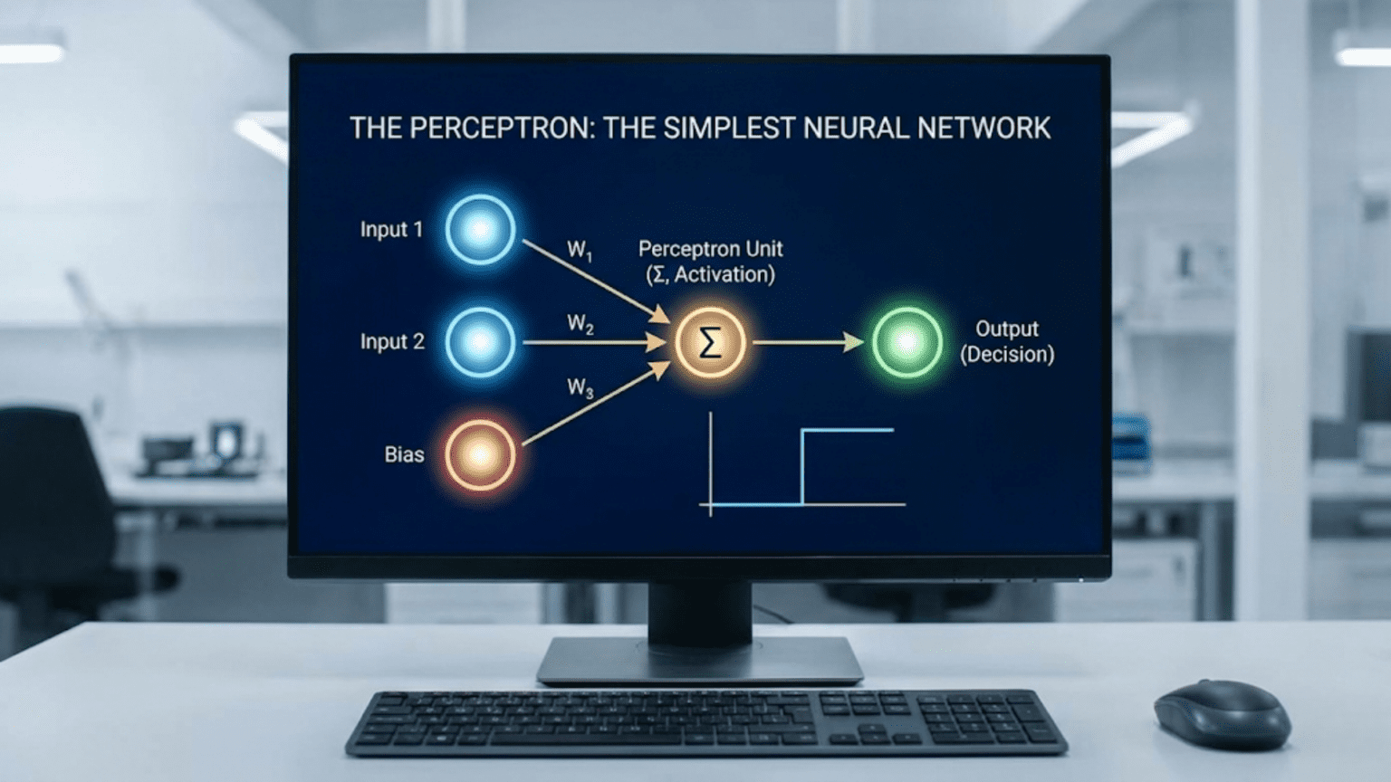
A perceptron is a single-layer neural network—the simplest possible architecture that can learn.
The Structure
Components:
1. Input Layer (x₁, x₂, …, xₙ):
- Multiple input values
- Features describing the example
- Numerical values
2. Weights (w₁, w₂, …, wₙ):
- One weight per input
- Determines input importance
- Learned during training
- Can be positive or negative
3. Bias (b):
- Additional learnable parameter
- Shifts the decision boundary
- Like an intercept in linear equations
4. Summation Function:
- Weighted sum of inputs plus bias
- z = w₁x₁ + w₂x₂ + … + wₙxₙ + b
5. Activation Function:
- Applies threshold
- Produces final output
- Typically step function (0 or 1)
6. Output (ŷ):
- Binary prediction
- Usually 0 or 1 (or -1 and +1)
- Single value
Visual Representation
Inputs          Weights        Summation      Activation    Output

x₁ ─────────────→ w₁ ─┐
                      │
x₂ ─────────────→ w₂ ─┤
                      ├─→     Σ(wᵢxᵢ + b)  ──→  f(z)  ────→   ŷ
x₃ ─────────────→ w₃ ─┤
                      │
b ──────────────→ 1 ──┘Mathematical Formula
Step 1: Weighted Sum
z = w₁x₁ + w₂x₂ + ... + wₙxₙ + b
= Σ(wᵢxᵢ) + bStep 2: Activation (Step Function)
ŷ = f(z) = {1 if z ≥ 0
{0 if z < 0Or sometimes:
ŷ = {+1 if z ≥ 0
{-1 if z < 0Simple Example
Problem: Classify if a student passes (1) or fails (0) based on study hours and sleep hours
Input Features:
- x₁ = study hours (0-10)
- x₂ = sleep hours (0-10)
Perceptron Parameters (learned):
- w₁ = 0.5 (weight for study hours)
- w₂ = 0.3 (weight for sleep hours)
- b = -3 (bias)
Prediction for New Student:
Student: study=6 hours, sleep=8 hours

z = (0.5 × 6) + (0.3 × 8) + (-3)
z = 3 + 2.4 - 3
z = 2.4

ŷ = f(2.4) = 1 (since 2.4 ≥ 0)

Prediction: PassThe Perceptron Learning Algorithm
How does the perceptron learn the right weights? Through a simple but powerful algorithm.
The Learning Process
Goal: Adjust weights so predictions match actual labels
Principle: Update weights based on errors
Algorithm:
1. Initialize weights randomly (or to zero)
2. For each training example (x, y):
   a. Make prediction: ŷ = f(Σwᵢxᵢ + b)
   b. Calculate error: error = y - ŷ
   c. Update each weight: wᵢ = wᵢ + η × error × xᵢ
   d. Update bias: b = b + η × error
3. Repeat until convergence (or max iterations)Where:
- η (eta) = learning rate (controls step size)
- error = actual – predicted
- If correct (error=0): weights unchanged
- If wrong (error≠0): weights adjusted
Learning Rule Intuition
Case 1: Correct Prediction
Actual: 1, Predicted: 1
Error: 1 - 1 = 0
Update: wᵢ = wᵢ + η × 0 × xᵢ = wᵢ (no change)

Weights stay the same—already working!Case 2: False Negative (should be 1, predicted 0)
Actual: 1, Predicted: 0
Error: 1 - 0 = 1
Update: wᵢ = wᵢ + η × 1 × xᵢ

If xᵢ > 0: weight increases (strengthens positive contribution)
If xᵢ < 0: weight decreases (reduces negative contribution)

Result: Next time, more likely to predict 1Case 3: False Positive (should be 0, predicted 1)
Actual: 0, Predicted: 1
Error: 0 - 1 = -1
Update: wᵢ = wᵢ + η × (-1) × xᵢ

If xᵢ > 0: weight decreases (reduces positive contribution)
If xᵢ < 0: weight increases (adds negative contribution)

Result: Next time, more likely to predict 0Step-by-Step Example
Problem: Learn AND gate (binary logic)
Training Data:
x₁  x₂  y (AND)
0   0   0
0   1   0
1   0   0
1 1 1Initialization:
w₁ = 0, w₂ = 0, b = 0
η = 0.1 (learning rate)Iteration 1, Example 1: x₁=0, x₂=0, y=0
z = (0×0) + (0×0) + 0 = 0
ŷ = f(0) = 1 (step function: 1 if z≥0)
error = 0 - 1 = -1

w₁ = 0 + 0.1×(-1)×0 = 0
w₂ = 0 + 0.1×(-1)×0 = 0
b = 0 + 0.1×(-1) = -0.1

New: w₁=0, w₂=0, b=-0.1Iteration 1, Example 2: x₁=0, x₂=1, y=0
z = (0×0) + (0×1) + (-0.1) = -0.1
ŷ = f(-0.1) = 0
error = 0 - 0 = 0

No update (correct prediction)
Weights: w₁=0, w₂=0, b=-0.1Iteration 1, Example 3: x₁=1, x₂=0, y=0
z = (0×1) + (0×0) + (-0.1) = -0.1
ŷ = f(-0.1) = 0
error = 0 - 0 = 0

No update
Weights: w₁=0, w₂=0, b=-0.1Iteration 1, Example 4: x₁=1, x₂=1, y=1
z = (0×1) + (0×1) + (-0.1) = -0.1
ŷ = f(-0.1) = 0
error = 1 - 0 = 1

w₁ = 0 + 0.1×1×1 = 0.1
w₂ = 0 + 0.1×1×1 = 0.1
b = -0.1 + 0.1×1 = 0

New: w₁=0.1, w₂=0.1, b=0Continue iterations until all predictions correct…
Final Learned Weights (after convergence):
w₁ ≈ 0.5, w₂ ≈ 0.5, b ≈ -0.7Verify:
(0,0): z = 0.5×0 + 0.5×0 - 0.7 = -0.7 → ŷ=0 ✓
(0,1): z = 0.5×0 + 0.5×1 - 0.7 = -0.2 → ŷ=0 ✓
(1,0): z = 0.5×1 + 0.5×0 - 0.7 = -0.2 → ŷ=0 ✓
(1,1): z = 0.5×1 + 0.5×1 - 0.7 = 0.3 → ŷ=1 ✓Perfect! The perceptron learned the AND function.
Geometric Interpretation: Decision Boundaries
The perceptron learns a linear decision boundary that separates classes.
Two-Dimensional Case
Perceptron Equation: w₁x₁ + w₂x₂ + b = 0
This is the equation of a line!
Decision Boundary: Line where z = 0
- Points where w₁x₁ + w₂x₂ + b = 0
- Separates positive and negative predictions
Classification:
- Above line (z > 0): Class 1
- Below line (z < 0): Class 0
- On line (z = 0): Boundary
Example Visualization (AND gate):
x₂
│
1 │     ○        ● (1,1) → 1
  │
  │ ○       ○
0 │_______________x₁
  0              1

Decision boundary: 0.5x₁ + 0.5x₂ - 0.7 = 0
Simplifies to: x₁ + x₂ = 1.4

○ = Class 0 (below line)
● = Class 1 (above line)What Perceptron Learns
During Training:
- Starts with random line (random weights)
- Adjusts line to separate classes
- Rotates and shifts boundary
- Stops when all points correctly classified
Weights Control:
- w₁, w₂: Slope/orientation of line
- b: Position (shifts line)
Learning = Finding Right Line:
- Line that separates positive and negative examples
- Minimizes classification errors
Higher Dimensions
3D (Three Inputs):
- Decision boundary = Plane
- w₁x₁ + w₂x₂ + w₃x₃ + b = 0
n Dimensions:
- Decision boundary = Hyperplane
- w₁x₁ + w₂x₂ + … + wₙxₙ + b = 0
Principle: Perceptron always learns linear decision boundary
The Perceptron Convergence Theorem
Powerful Guarantee: If data is linearly separable, the perceptron will find a solution in finite steps.
Linearly Separable
Definition: Two classes can be perfectly separated by a straight line (or hyperplane)
Linearly Separable Examples:
- AND gate: Can draw line separating 0s and 1s
- OR gate: Can separate classes
- Simple binary classification with clear separation
NOT Linearly Separable:
- XOR gate: No line can separate (we’ll see why this matters)
- Concentric circles
- Interleaved patterns
Convergence Theorem (Rosenblatt, 1958):
IF data is linearly separable
THEN perceptron will converge to a solution in finite steps

Steps bounded by: (R/γ)²
Where:
- R = maximum distance of any point from origin
- γ = margin (minimum distance from points to optimal hyperplane)Practical Implication:
- Linearly separable → guaranteed convergence
- Not linearly separable → will never converge, oscillates forever
Limitations of the Perceptron
Despite its elegance, the perceptron has fundamental limitations.
Limitation 1: Only Linear Boundaries
Problem: Can only learn linear decision boundaries
Consequence: Cannot solve non-linearly separable problems
Famous Example: XOR Problem
XOR Truth Table:
x₁  x₂  y (XOR)
0   0   0
0   1   1
1   0   1
1 1 0Visualization:
x₂
│
1 │  1        0
  │
  │  0        1
0 │___________x₁
0 1Problem: No straight line separates 1s from 0s!
- Any line that puts (0,1) and (1,0) on one side also captures (0,0) or (1,1)
- Fundamentally impossible for single perceptron
Historical Impact:
- Marvin Minsky and Seymour Papert’s 1969 book “Perceptrons” highlighted this limitation
- Caused “AI Winter”—funding and interest in neural networks dried up
- Not overcome until multi-layer networks in 1980s
Limitation 2: Binary Output Only
Problem: Single perceptron produces only binary output
Consequence: Cannot solve:
- Multi-class classification (more than 2 classes)
- Regression (continuous values)
- Probability estimates
Workarounds:
- Multi-class: One perceptron per class
- Continuous: Different activation function (but then not classic perceptron)
Limitation 3: No Hidden Representations
Problem: No intermediate layers to learn features
Consequence:
- Must work with given features
- Cannot learn feature combinations
- Cannot discover abstract representations
Example:
Given: Raw pixel values
Can't learn: "This is an edge" or "this is a curve"
Limited to: Direct pixel-to-class mappingLimitation 4: Sensitive to Outliers
Problem: Perceptron tries to classify all points correctly
Consequence: Single outlier can significantly affect decision boundary
No Margin Maximization: Unlike SVM, doesn’t maximize separation margin
Limitation 5: No Probabilistic Output
Problem: Output is hard 0 or 1
Consequence: No confidence estimates
- Can’t say “90% confident this is class 1”
- Just binary prediction
Modern Solution: Use sigmoid activation (becomes logistic regression)
From Perceptron to Modern Neural Networks
The perceptron evolved into sophisticated neural networks.
Evolution 1: Multi-Layer Perceptron (MLP)
Key Innovation: Add hidden layers
Architecture:
Input → Hidden Layer 1 → Hidden Layer 2 → Output
Solves: XOR and other non-linear problems
- Hidden layers create non-linear decision boundaries
- Can approximate any continuous function (universal approximation theorem)
XOR Solution with 2-Layer Network:
Input Layer (2) → Hidden Layer (2) → Output Layer (1)

Hidden layer learns:
- Neuron 1: Detects x₁ OR x₂
- Neuron 2: Detects x₁ AND x₂

Output combines:
- Output = (x₁ OR x₂) AND NOT(x₁ AND x₂)
- This is XOR!Evolution 2: Different Activation Functions
Beyond Step Function:
Sigmoid: σ(z) = 1/(1 + e^(-z))
- Smooth, differentiable
- Outputs probabilities (0 to 1)
- Enables gradient-based learning
Tanh: tanh(z) = (e^z – e^(-z))/(e^z + e^(-z))
- Similar to sigmoid
- Outputs -1 to 1
- Often works better than sigmoid
ReLU: f(z) = max(0, z)
- Modern standard for deep networks
- Faster training
- Reduces vanishing gradient problem
Impact: Smooth activations enable backpropagation
Evolution 3: Backpropagation
Beyond Perceptron Learning Rule:
Problem: Perceptron rule doesn’t work for multi-layer networks
- Can’t directly compute error for hidden layers
Solution: Backpropagation (1986)
- Compute gradient of error with respect to weights
- Propagate error backward through network
- Update all weights using gradient descent
Impact: Enabled training deep networks
Evolution 4: Continuous Outputs
Regression:
- Use linear activation (no threshold)
- Predict continuous values
Multi-class Classification:
- Multiple output neurons
- Softmax activation
- Probability distribution over classes
Evolution 5: Specialized Architectures
Convolutional Neural Networks (CNNs):
- Specialized for images
- Convolutional layers detect local patterns
- Built from perceptron-like units
Recurrent Neural Networks (RNNs):
- Feedback connections
- Process sequences
- Memory of past inputs
Transformers:
- Attention mechanisms
- Parallel processing
- Modern NLP standard
Foundation: All build on perceptron’s core idea
Implementing a Perceptron
Let’s build a perceptron from scratch to solidify understanding.
Python Implementation
import numpy as np

class Perceptron:
    def __init__(self, learning_rate=0.1, n_iterations=100):
        self.lr = learning_rate
        self.n_iterations = n_iterations
        self.weights = None
        self.bias = None

    def fit(self, X, y):
        """Train the perceptron"""
        n_samples, n_features = X.shape

        # Initialize weights and bias to zero
        self.weights = np.zeros(n_features)
        self.bias = 0

        # Convert y to -1 and 1 (if not already)
        y_ = np.where(y <= 0, -1, 1)

        # Training loop
        for _ in range(self.n_iterations):
            for idx, x_i in enumerate(X):
                # Prediction
                linear_output = np.dot(x_i, self.weights) + self.bias
                y_predicted = np.where(linear_output >= 0, 1, -1)

                # Update if wrong
                if y_[idx] * y_predicted <= 0:  # Misclassified
                    update = self.lr * y_[idx]
                    self.weights += update * x_i
                    self.bias += update

    def predict(self, X):
        """Make predictions"""
        linear_output = np.dot(X, self.weights) + self.bias
        return np.where(linear_output >= 0, 1, -1)

# Example: AND gate
X = np.array([[0, 0], [0, 1], [1, 0], [1, 1]])
y = np.array([0, 0, 0, 1])

perceptron = Perceptron(learning_rate=0.1, n_iterations=10)
perceptron.fit(X, y)

print("Learned weights:", perceptron.weights)
print("Learned bias:", perceptron.bias)
print("Predictions:", perceptron.predict(X))Using Scikit-learn
from sklearn.linear_model import Perceptron
from sklearn.datasets import make_classification
from sklearn.model_selection import train_test_split

# Generate linearly separable data
X, y = make_classification(n_samples=100, n_features=2, n_redundant=0,
                          n_informative=2, n_clusters_per_class=1)

# Split data
X_train, X_test, y_train, y_test = train_test_split(X, y, test_size=0.2)

# Train perceptron
perceptron = Perceptron(max_iter=100, eta0=0.1, random_state=42)
perceptron.fit(X_train, y_train)

# Evaluate
accuracy = perceptron.score(X_test, y_test)
print(f"Accuracy: {accuracy:.2f}")

# Weights and bias
print("Weights:", perceptron.coef_)
print("Bias:", perceptron.intercept_)Historical Significance and Legacy
The perceptron’s impact extends far beyond its technical capabilities.
1958: The Mark I Perceptron
Frank Rosenblatt’s Achievement:
- First hardware implementation
- 400 photocells as “retina”
- Learned to distinguish simple shapes
- Demonstrated machine learning in action
Media Hype:
- New York Times coverage
- Predictions of thinking machines
- Public excitement about AI
Reality:
- Could solve simple problems
- Demonstrated learning from examples
- Showed promise of neural approaches
1969: “AI Winter”
Minsky and Papert’s Book:
- Mathematically proved perceptron limitations
- XOR problem unsolvable by single perceptron
- Highlighted what perceptrons cannot do
Impact:
- Funding dried up
- Research interest declined
- Neural networks largely abandoned
Unfair Critique:
- Multi-layer networks could solve XOR
- But training methods not yet developed
- Focus on limitations rather than potential
1980s: Renaissance
Backpropagation Discovery (1986):
- Rumelhart, Hinton, Williams
- Training method for multi-layer networks
- Overcame perceptron limitations
Renewed Interest:
- Multi-layer perceptrons (MLPs) powerful
- Could learn non-linear boundaries
- Universal function approximators
Modern Era: Foundation of Deep Learning
Legacy:
- Every neuron in deep networks is perceptron-like
- Core concepts persist:
- Weighted sums
- Learnable parameters
- Threshold/activation
- Error-driven learning
Evolution:
- Deeper networks (100+ layers)
- Better activations (ReLU vs step)
- Advanced optimization (Adam vs perceptron rule)
- Specialized architectures (CNN, Transformer)
But Fundamentally: Same basic building block
Practical Applications of Perceptrons
Where perceptrons (and linear classifiers) still useful:
Use Case 1: Simple Binary Classification
When Appropriate:
- Linearly separable data
- Need interpretability
- Fast training required
- Limited data
Examples:
- Spam vs. not spam (with good features)
- Sentiment: positive vs. negative
- Pass vs. fail (with clear criteria)
Use Case 2: Online Learning
Advantage: Can update one example at a time
Applications:
- Streaming data
- Adaptive systems
- Real-time learning
Example: Email spam filter that learns from user feedback
Use Case 3: Ensemble Component
Use: Perceptrons as weak learners in ensembles
Methods:
- Boosting: Combine multiple perceptrons
- Voting: Ensemble of perceptron variants
Use Case 4: Feature Selection
Use: Perceptron weights indicate feature importance
Process:
- Train perceptron
- Examine weights
- Large weights → important features
- Small weights → unimportant features
Use Case 5: Teaching Tool
Perfect For:
- Learning neural network basics
- Understanding gradient-free learning
- Visualizing decision boundaries
- Implementing from scratch
Comparison: Perceptron vs. Modern Methods
| Aspect | Perceptron | Multi-Layer NN | Logistic Regression | SVM |
|---|---|---|---|---|
| Architecture | Single neuron | Multiple layers | Single neuron | Kernel methods |
| Decision Boundary | Linear | Non-linear possible | Linear | Non-linear with kernels |
| Activation | Step function | ReLU, sigmoid, etc. | Sigmoid | N/A (different approach) |
| Output | Binary (0/1) | Continuous/multi-class | Probability (0-1) | Binary/continuous |
| Learning | Perceptron rule | Backpropagation | Gradient descent | Quadratic programming |
| Can Solve XOR | No | Yes | No | Yes (with kernel) |
| Convergence | Guaranteed if separable | Not guaranteed | Guaranteed | Guaranteed |
| Interpretability | High | Low | High | Medium |
| Speed | Very fast | Slower | Fast | Medium |
| Best For | Simple, linearly separable | Complex patterns | Probabilistic classification | Max-margin classification |
Conclusion: Simple Yet Profound
The perceptron stands as one of the most elegant ideas in machine learning. A single artificial neuron that learns from examples, adjusting weights based on errors until it correctly classifies linearly separable patterns. Simple to understand, simple to implement, yet sophisticated enough to demonstrate the core principles of neural learning.
Its limitations—inability to solve XOR, restriction to linear boundaries, binary outputs—ultimately proved as instructive as its capabilities. These limitations motivated the development of multi-layer networks, backpropagation, and eventually deep learning. The perceptron’s failure to solve XOR launched research that eventually enabled networks to master far more complex tasks.
Understanding the perceptron provides essential foundation for neural networks:
Core concepts introduced:
- Weighted inputs representing importance
- Learnable parameters adjusted by experience
- Threshold-based activation
- Error-driven learning
- Geometric interpretation as decision boundaries
Limitations that drove progress:
- Need for hidden layers (multi-layer networks)
- Need for smooth activations (sigmoid, ReLU)
- Need for better learning algorithms (backpropagation)
- Need for non-linear boundaries (deep learning)
Every modern deep neural network—whether classifying images, translating languages, or playing games—consists of perceptron-like units connected in sophisticated architectures, trained with advanced algorithms, but fundamentally built on the same principles Rosenblatt demonstrated in 1958.
The perceptron’s journey from breakthrough to limitation to foundation teaches an important lesson about AI progress: sometimes the most valuable contributions aren’t perfect solutions but rather elegant ideas that reveal both what’s possible and what’s needed next. The perceptron showed that machines could learn from examples, demonstrated the power and limits of single-layer networks, and established principles that remain relevant sixty years later.
As you continue learning about neural networks, remember that every complex architecture you encounter builds on this simple foundation: artificial neurons receiving weighted inputs, computing sums, passing through activations, and learning from errors. Master the perceptron, and you’ve mastered the fundamental building block of all neural networks.