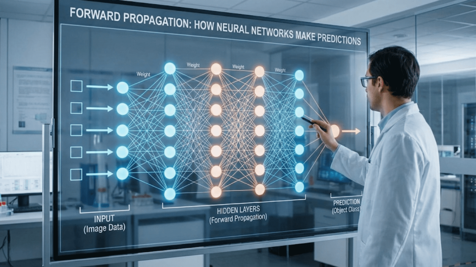
Forward propagation is the process by which neural networks make predictions by passing input data through successive layers, computing weighted sums and applying activation functions at each neuron, until producing a final output. Information flows in one direction—forward from input layer through hidden layers to output layer—with each layer transforming the data based on learned weights and biases. This forward pass converts raw inputs into predictions, whether classifying images, translating text, or making any other prediction the network was trained for.
Introduction: The Journey from Input to Output
Imagine water flowing through a series of filters and treatment stages at a water processing plant. Raw water enters, passes through sedimentation tanks, filtration systems, and chemical treatments, with each stage transforming the water until clean, drinkable water emerges at the end. Neural network prediction works similarly: raw data enters the input layer, flows through hidden layers where it’s progressively transformed, and emerges as a prediction at the output layer.
This process—forward propagation—is how neural networks actually make predictions. It’s the “forward” in “feedforward neural networks” and the mechanism behind every prediction a trained network makes. Whether classifying an image as a cat or dog, translating a sentence, recommending a product, or playing a game move, forward propagation is the computational pipeline that converts inputs into outputs.
Understanding forward propagation is essential for anyone working with neural networks. It’s not just theoretical—this is literally what happens every time you use a neural network. When you upload a photo to identify faces, forward propagation runs. When you ask a chatbot a question, forward propagation computes the response. When a self-driving car interprets sensor data, forward propagation processes it.
Moreover, understanding forward propagation is crucial for debugging networks, optimizing performance, and grasping how learning (backpropagation) works. You can’t fully understand how networks learn without first understanding how they make predictions.
This comprehensive guide walks through forward propagation step-by-step. You’ll learn the mathematical operations at each layer, trace a complete example from input to output, understand the role of weights and biases, see how activation functions transform data, explore matrix operations that make it efficient, and gain practical intuition for what’s happening inside neural networks when they predict.
What is Forward Propagation?
Forward propagation (also called forward pass) is the process of computing the output of a neural network by passing input data through the network layer by layer.
The Basic Concept
Information Flow:
Input → Layer 1 → Layer 2 → ... → Layer N → Output

Data flows in one direction: forward (input to output)
No backward flow during predictionAt Each Layer:
- Receive inputs from previous layer
- Compute weighted sum of inputs
- Add bias
- Apply activation function
- Pass output to next layer
Complete Process:
Input values
→ Multiply by weights, add biases (Layer 1)
→ Apply activation function (Layer 1)
→ Multiply by weights, add biases (Layer 2)
→ Apply activation function (Layer 2)
→ ...
→ Final output/predictionWhy “Propagation”?
Propagate: To spread or transmit through a medium
In Neural Networks: Information propagates (spreads) through the network
- Starts at input layer
- Transmits through hidden layers
- Reaches output layer
Signal Flow: Like electrical signal through circuit or sound wave through air
- Each layer receives signal
- Transforms it
- Passes it forward
The Mathematics: Step-by-Step
Let’s break down the exact calculations at each neuron and layer.
Single Neuron Computation
For one neuron:
Inputs: x₁, x₂, …, xₙ
Weights: w₁, w₂, …, wₙ
Bias: b
Step 1: Weighted Sum (Linear Transformation)
z = w₁x₁ + w₂x₂ + ... + wₙxₙ + b
z = Σ(wᵢxᵢ) + bStep 2: Activation Function (Non-linear Transformation)
a = f(z)

Where f is the activation function (ReLU, sigmoid, etc.)Output: a (activation value, passed to next layer)
Layer Computation
For a layer with multiple neurons:
Each neuron independently computes weighted sum and activation.
Example: Layer with 3 neurons
Inputs: x₁, x₂ (2 inputs)
Neuron 1:
z₁ = w₁₁x₁ + w₁₂x₂ + b₁
a₁ = f(z₁)Neuron 2:
z₂ = w₂₁x₁ + w₂₂x₂ + b₂
a₂ = f(z₂)Neuron 3:
z₃ = w₃₁x₁ + w₃₂x₂ + b₃
a₃ = f(z₃)Layer Output: [a₁, a₂, a₃]
Multi-Layer Network
General Formula for Layer l:
Z⁽ˡ⁾ = W⁽ˡ⁾A⁽ˡ⁻¹⁾ + b⁽ˡ⁾
A⁽ˡ⁾ = f⁽ˡ⁾(Z⁽ˡ⁾)

Where:
- l = layer number
- Z⁽ˡ⁾ = weighted sums for layer l
- W⁽ˡ⁾ = weight matrix for layer l
- A⁽ˡ⁻¹⁾ = activations from previous layer (layer l-1)
- b⁽ˡ⁾ = bias vector for layer l
- f⁽ˡ⁾ = activation function for layer l
- A⁽ˡ⁾ = activations for layer lFor Input Layer:
A⁽⁰⁾ = X (input data)Forward Propagation Algorithm:
For l = 1 to L (number of layers):
    Z⁽ˡ⁾ = W⁽ˡ⁾A⁽ˡ⁻¹⁾ + b⁽ˡ⁾
    A⁽ˡ⁾ = f⁽ˡ⁾(Z⁽ˡ⁾)

Output: A⁽ᴸ⁾ (final layer activation = prediction)Complete Example: Step-by-Step Walkthrough
Let’s trace forward propagation through a simple network.
Network Architecture
Task: Binary classification (0 or 1)
Architecture:
- Input layer: 2 neurons (2 features)
- Hidden layer: 3 neurons (ReLU activation)
- Output layer: 1 neuron (sigmoid activation)
Input (2) → Hidden (3) → Output (1)Given Parameters
Input:
x₁ = 0.5
x₂ = 0.8
X = [0.5, 0.8]Layer 1 (Input → Hidden) Weights:
W⁽¹⁾ = [0.2   0.5]
       [0.3  -0.2]
       [0.1   0.4]

b⁽¹⁾ = [0.1]
       [0.2]
[0.3]Layer 2 (Hidden → Output) Weights:
W⁽²⁾ = [0.5  -0.3  0.6]

b⁽²⁾ = [0.1]Layer 1: Input → Hidden
Step 1: Compute Weighted Sums
Neuron 1:
z₁⁽¹⁾ = (0.2 × 0.5) + (0.5 × 0.8) + 0.1
     = 0.1 + 0.4 + 0.1
= 0.6Neuron 2:
z₂⁽¹⁾ = (0.3 × 0.5) + (-0.2 × 0.8) + 0.2
     = 0.15 - 0.16 + 0.2
= 0.19Neuron 3:
z₃⁽¹⁾ = (0.1 × 0.5) + (0.4 × 0.8) + 0.3
     = 0.05 + 0.32 + 0.3
= 0.67Z⁽¹⁾ = [0.6, 0.19, 0.67]
Step 2: Apply Activation (ReLU)
ReLU(z) = max(0, z)

a₁⁽¹⁾ = ReLU(0.6) = 0.6
a₂⁽¹⁾ = ReLU(0.19) = 0.19
a₃⁽¹⁾ = ReLU(0.67) = 0.67

A⁽¹⁾ = [0.6, 0.19, 0.67]Layer 2: Hidden → Output
Step 1: Compute Weighted Sum
z⁽²⁾ = (0.5 × 0.6) + (-0.3 × 0.19) + (0.6 × 0.67) + 0.1
    = 0.3 - 0.057 + 0.402 + 0.1
= 0.745Step 2: Apply Activation (Sigmoid)
σ(z) = 1 / (1 + e^(-z))

a⁽²⁾ = σ(0.745)
    = 1 / (1 + e^(-0.745))
    = 1 / (1 + 0.475)
    = 1 / 1.475
    = 0.678

A⁽²⁾ = 0.678Final Prediction
Output: 0.678
Interpretation (for binary classification):
- Probability of class 1: 67.8%
- If threshold = 0.5: Predict class 1
- If threshold = 0.7: Predict class 0
Complete Forward Pass Summary:
Input: [0.5, 0.8]
↓
Layer 1 (ReLU): [0.6, 0.19, 0.67]
↓
Layer 2 (Sigmoid): 0.678
↓
Prediction: Class 1 (67.8% confidence)Matrix Notation: Efficient Computation
For practical implementation, we use matrix operations.
Why Matrices?
Advantages:
- Compact notation
- Efficient computation (vectorized)
- GPU acceleration
- Handles multiple examples simultaneously (batches)
Single Example
Layer l:
Z⁽ˡ⁾ = W⁽ˡ⁾A⁽ˡ⁻¹⁾ + b⁽ˡ⁾
A⁽ˡ⁾ = f(Z⁽ˡ⁾)

Dimensions:
- W⁽ˡ⁾: (n⁽ˡ⁾ × n⁽ˡ⁻¹⁾) - rows = neurons in layer l, cols = neurons in layer l-1
- A⁽ˡ⁻¹⁾: (n⁽ˡ⁻¹⁾ × 1) - activations from previous layer
- b⁽ˡ⁾: (n⁽ˡ⁾ × 1) - biases for layer l
- Z⁽ˡ⁾: (n⁽ˡ⁾ × 1) - weighted sums
- A⁽ˡ⁾: (n⁽ˡ⁾ × 1) - activationsExample (from above):
Layer 1:
W⁽¹⁾ (3×2) × A⁽⁰⁾ (2×1) + b⁽¹⁾ (3×1) = Z⁽¹⁾ (3×1)

[0.2   0.5]     [0.5]   [0.1]   [0.6 ]
[0.3  -0.2]  ×  [0.8] + [0.2] = [0.19]
[0.1 0.4] [0.3] [0.67]Batch Processing
Multiple Examples Simultaneously:
Z⁽ˡ⁾ = W⁽ˡ⁾A⁽ˡ⁻¹⁾ + b⁽ˡ⁾

Dimensions (m examples):
- W⁽ˡ⁾: (n⁽ˡ⁾ × n⁽ˡ⁻¹⁾) - same as before
- A⁽ˡ⁻¹⁾: (n⁽ˡ⁻¹⁾ × m) - each column is one example
- b⁽ˡ⁾: (n⁽ˡ⁾ × 1) - broadcast across all examples
- Z⁽ˡ⁾: (n⁽ˡ⁾ × m) - each column is one example's weighted sumsExample (3 examples, batch size = 3):
X = [0.5  0.2  0.8]  (2 features, 3 examples)
    [0.8  0.6  0.3]

Layer 1:
W⁽¹⁾ (3×2) × X (2×3) + b⁽¹⁾ (3×1) = Z⁽¹⁾ (3×3)

Each column of Z⁽¹⁾ corresponds to one example
All computed in single matrix operation (efficient!)Implementation: Python Code
NumPy Implementation
import numpy as np

def sigmoid(z):
    return 1 / (1 + np.exp(-z))

def relu(z):
    return np.maximum(0, z)

def forward_propagation(X, parameters):
    """
    Forward propagation for a 2-layer network

    Arguments:
    X -- input data (n_x, m) where m is number of examples
    parameters -- dict containing W1, b1, W2, b2

    Returns:
    A2 -- output of the network
    cache -- dict containing Z1, A1, Z2, A2 (for backpropagation)
    """
    # Retrieve parameters
    W1 = parameters['W1']
    b1 = parameters['b1']
    W2 = parameters['W2']
    b2 = parameters['b2']

    # Layer 1
    Z1 = np.dot(W1, X) + b1      # Weighted sum
    A1 = relu(Z1)                 # Activation

    # Layer 2
    Z2 = np.dot(W2, A1) + b2     # Weighted sum
    A2 = sigmoid(Z2)              # Activation

    # Store values for backpropagation
    cache = {
        'Z1': Z1,
        'A1': A1,
        'Z2': Z2,
        'A2': A2
    }

    return A2, cache

# Example usage
X = np.array([[0.5], [0.8]])  # Single example

parameters = {
    'W1': np.array([[0.2, 0.5],
                    [0.3, -0.2],
                    [0.1, 0.4]]),
    'b1': np.array([[0.1], [0.2], [0.3]]),
    'W2': np.array([[0.5, -0.3, 0.6]]),
    'b2': np.array([[0.1]])
}

prediction, cache = forward_propagation(X, parameters)
print(f"Prediction: {prediction[0][0]:.3f}")
# Output: Prediction: 0.678Deep Network (L layers)
def forward_propagation_deep(X, parameters, activations):
    """
    Forward propagation for L-layer network

    Arguments:
    X -- input data (n_x, m)
    parameters -- dict containing W1, b1, W2, b2, ..., WL, bL
    activations -- list of activation functions for each layer

    Returns:
    AL -- output of the network
    caches -- list of caches for each layer
    """
    caches = []
    A = X
    L = len(parameters) // 2  # Number of layers

    # Loop through layers
    for l in range(1, L + 1):
        A_prev = A

        # Retrieve parameters
        W = parameters[f'W{l}']
        b = parameters[f'b{l}']

        # Forward step
        Z = np.dot(W, A_prev) + b
        A = activations[l-1](Z)

        # Store cache
        cache = {
            'A_prev': A_prev,
            'W': W,
            'b': b,
            'Z': Z,
            'A': A
        }
        caches.append(cache)

    return A, caches

# Example: 3-layer network
parameters = {
    'W1': np.random.randn(4, 2) * 0.01,
    'b1': np.zeros((4, 1)),
    'W2': np.random.randn(3, 4) * 0.01,
    'b2': np.zeros((3, 1)),
    'W3': np.random.randn(1, 3) * 0.01,
    'b3': np.zeros((1, 1))
}

activations = [relu, relu, sigmoid]  # ReLU for hidden, sigmoid for output

AL, caches = forward_propagation_deep(X, parameters, activations)TensorFlow/Keras
import tensorflow as tf
from tensorflow import keras

# Define model
model = keras.Sequential([
    keras.layers.Dense(3, activation='relu', input_shape=(2,)),
    keras.layers.Dense(1, activation='sigmoid')
])

# Forward propagation happens automatically
X = np.array([[0.5, 0.8]])
prediction = model(X)
print(prediction)Visualizing Forward Propagation
Network Diagram with Values
Input Layer    Hidden Layer    Output Layer
              (ReLU)          (Sigmoid)

  0.5 ────────→ 0.6 ─────────┐
            ╱   0.19 ────────┤
  0.8 ────╱     0.67 ────────┴→ 0.678
         ╲
          ╲
           ╲

Values flow left to right
Each connection has a weight
Each neuron computes weighted sum + bias
Then applies activation functionData Transformation View
Input Space          Hidden Space         Output Space
(2D)                (3D)                 (1D)

[0.5, 0.8] ─────→ [0.6, 0.19, 0.67] ─────→ 0.678

Original            Transformed          Final
features representation predictionEach layer:
- Projects data into different dimensional space
- Learns useful representation
- Extracts features
Common Patterns and Architectures
Feedforward (Fully Connected)
Structure: Every neuron in layer l connects to every neuron in layer l+1
Forward Pass: Standard process described above
Use Cases:
- General purpose
- Tabular data
- Smaller datasets
Convolutional Neural Networks (CNNs)
Structure: Convolutional layers + pooling layers
Forward Pass:
- Convolutional layer: Apply filters to input
- Pooling layer: Downsample (max or average pooling)
- Flatten → Fully connected layers
Use Cases: Images, spatial data
Recurrent Neural Networks (RNNs)
Structure: Recurrent connections (feedback loops)
Forward Pass:
- Process sequence step-by-step
- Hidden state carried forward
- Each step: combine current input with previous hidden state
Use Cases: Sequences, time series, text
Forward Propagation in Training vs. Inference
During Training
Purpose:
- Compute predictions
- Calculate loss
- Enable backpropagation
Process:
1. Forward propagation → predictions
2. Calculate loss (prediction vs. actual)
3. Backpropagation → gradients
4. Update weights
5. RepeatStore Intermediate Values: Need Z and A for each layer (for backpropagation)
During Inference (Prediction)
Purpose: Make predictions on new data
Process:
1. Forward propagation → predictions
2. Return predictionsDon’t Need:
- Intermediate values (no backpropagation)
- Gradients
- Weight updates
Optimizations:
- Drop dropout layers (only for training)
- Use batch normalization in inference mode
- Can simplify architecture
Key Concepts and Insights
1. Layer-by-Layer Transformation
Each layer transforms data representation:
- Input: Raw features
- Hidden Layer 1: Low-level features
- Hidden Layer 2: Mid-level features
- Hidden Layer 3: High-level features
- Output: Prediction
Example (Image Recognition):
Input: Pixels (raw)
Layer 1: Edges, textures
Layer 2: Parts (eyes, wheels)
Layer 3: Objects (faces, cars)
Output: Classification2. Weighted Voting
Each neuron performs weighted voting:
- Inputs vote with different strengths (weights)
- Positive weights: excitatory
- Negative weights: inhibitory
- Bias: threshold adjustment
3. Non-Linearity is Crucial
Activation functions enable:
- Complex decision boundaries
- Hierarchical features
- Universal function approximation
Without activation: Network collapses to linear model
4. Dimensionality Changes
Each layer can change dimensions:
- Expand: 10 inputs → 100 hidden neurons (learn richer representation)
- Compress: 100 → 10 (dimensionality reduction, bottleneck)
- Same: 50 → 50 (maintain dimensionality)
5. Parallel Computation
Within a layer:
- All neurons compute independently
- Can be parallelized (GPU advantage)
- Matrix operations enable efficiency
Debugging Forward Propagation
Common Issues
Issue 1: Dimension Mismatch
Error: "shapes (3,2) and (3,1) not aligned"

Problem: W shape incompatible with input shape
Solution: Check weight matrix dimensionsIssue 2: Exploding Activations
Warning: Activations become very large (>1000)

Problem: Poor initialization or missing activation
Solution: Proper weight initialization, check activationsIssue 3: Dead Neurons (ReLU)
Symptom: Many neurons always output 0

Problem: Negative inputs to ReLU
Solution: Check initialization, learning rate, use Leaky ReLUIssue 4: NaN Values
Error: Output contains NaN

Problem: Numerical instability (overflow in exp())
Solution: Gradient clipping, better initialization, normalize inputsDebugging Checklist
- Check Shapes: Verify matrix dimensions match
- Inspect Values: Print intermediate activations
- Verify Activations: Ensure activation functions applied
- Check Ranges: Look for exploding/vanishing values
- Test Small Example: Manual calculation to verify logic
Performance Considerations
Computational Complexity
Time Complexity: O(n² × L) where n = neurons per layer, L = layers
Space Complexity: O(n × L) for storing activations
Optimization Techniques
Vectorization:
- Use matrix operations (NumPy, TensorFlow)
- Avoid Python loops
- 100-1000x speedup
Batch Processing:
- Process multiple examples simultaneously
- Better GPU utilization
- Amortize overhead
Mixed Precision:
- Use float16 instead of float32
- Reduces memory, increases speed
- Minimal accuracy loss
GPU Acceleration:
- Parallel computation
- Specialized tensor cores
- 10-100x speedup over CPU
Comparison: Forward vs. Backward Propagation
| Aspect | Forward Propagation | Backpropagation |
|---|---|---|
| Direction | Input → Output | Output → Input |
| Purpose | Make predictions | Compute gradients |
| Computation | Z = WA + b, A = f(Z) | ∂L/∂W, ∂L/∂b |
| Used During | Training and inference | Training only |
| Stores | Activations (Z, A) | Gradients (dW, db) |
| Complexity | O(n²L) | O(n²L) (similar) |
| Output | Predictions | Weight updates |
Practical Example: Image Classification
Network for MNIST Digits
Input: 28×28 grayscale image (784 pixels) Output: 10 classes (digits 0-9)
Architecture:
Input (784) → Hidden 1 (128, ReLU) → Hidden 2 (64, ReLU) → Output (10, Softmax)
Forward Propagation:
# Flatten image
X = image.flatten()  # (784, 1)

# Layer 1
Z1 = W1 @ X + b1     # (128, 1)
A1 = relu(Z1)         # (128, 1)

# Layer 2
Z2 = W2 @ A1 + b2    # (64, 1)
A2 = relu(Z2)         # (64, 1)

# Output layer
Z3 = W3 @ A2 + b3    # (10, 1)
A3 = softmax(Z3)      # (10, 1) - probabilities for each digit

# Prediction
predicted_digit = argmax(A3) # Digit with highest probabilityExample Output:
A3 (probabilities):
[0.01, 0.02, 0.03, 0.65, 0.05, 0.08, 0.03, 0.01, 0.10, 0.02]
 0     1     2     3     4     5     6     7     8     9

Prediction: Digit 3 (65% confidence)Conclusion: The Foundation of Neural Network Predictions
Forward propagation is the fundamental mechanism by which neural networks transform inputs into predictions. Through a series of linear transformations (weighted sums) and non-linear activations, raw data flows through layers, with each layer learning increasingly abstract representations until producing a final prediction.
Understanding forward propagation deeply means grasping:
The mechanics: Weighted sums, bias additions, and activation functions at each neuron, computed layer by layer from input to output.
The mathematics: Matrix operations that efficiently compute forward passes for entire batches of data simultaneously.
The transformations: How each layer projects data into different spaces, learning useful representations that make the final prediction task easier.
The efficiency: How vectorization and parallelization enable networks to make thousands of predictions per second.
Forward propagation might seem straightforward—just multiply, add, activate, and repeat—but this simple process is what enables neural networks to recognize faces, understand language, play games, and solve complex problems. Every sophisticated AI application ultimately relies on this basic computation.
As you build and work with neural networks, remember that every prediction starts with forward propagation. Debug it carefully, optimize it for speed, and understand its limitations. It’s the first half of the learning process (the other being backpropagation), and mastering it is essential for effective deep learning.
The beauty of forward propagation lies in its simplicity and power: a straightforward algorithm that, when combined with the right architecture and sufficient training data, can learn to approximate virtually any function, enabling the remarkable AI capabilities we see today.