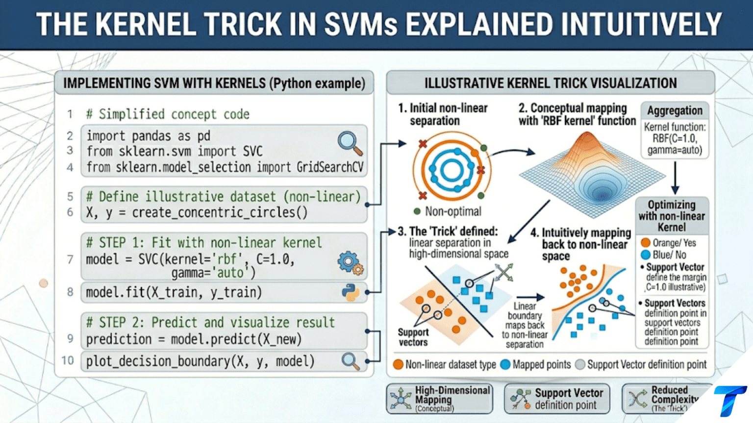
The kernel trick allows SVMs to find nonlinear decision boundaries without explicitly computing the high-dimensional feature transformation. Instead of mapping each data point to a new space and computing dot products there, a kernel function K(x, z) computes the dot product in the transformed space directly from the original features. This makes it computationally feasible to work in spaces with millions or even infinite dimensions, enabling SVMs to classify data with curved, circular, or arbitrarily complex boundaries.
Introduction
Article 79 showed that the SVM dual optimization depends only on dot products between training points: ∑_i,j α_i α_j y_i y_j x_i^T x_j. This innocent-looking observation is the doorway to the kernel trick — one of the most elegant ideas in machine learning.
The problem with linear SVMs is that they can only find straight-line (or hyperplane) boundaries. Many real problems have circular, elliptical, or more complex boundaries. One solution is to transform the data into a higher-dimensional space where it becomes linearly separable. For example, data arranged in two concentric circles in 2D might become linearly separable in 3D after adding a feature r² = x₁² + x₂².
The catch: these feature mappings can be enormous. The polynomial feature map of degree d applied to d-dimensional input has O(d^d) terms. For d = 100 and degree 3, that is a million features per sample. Even computing the transformation would be prohibitive, let alone training a model on it.
The kernel trick sidesteps this computation entirely. Because the SVM dual only needs dot products in the transformed space, and because certain functions K(x, z) compute this dot product directly without ever computing the transformation φ(x) explicitly, we can work in infinite-dimensional spaces with the computational cost of simple function evaluations.
This article builds the kernel trick from scratch: the feature map intuition, the Mercer condition that defines valid kernels, the most important kernel functions, kernel visualization, custom kernel implementation, and practical guidance on choosing the right kernel.
The Feature Map Intuition
Linear Inseparability and Feature Expansion
Some classification problems are not linearly separable in the original feature space but become separable after adding carefully chosen new features.
import numpy as np
import matplotlib.pyplot as plt
from sklearn.svm import SVC
from sklearn.datasets import make_circles
from sklearn.preprocessing import StandardScaler
import warnings
warnings.filterwarnings('ignore')

np.random.seed(42)


def demonstrate_feature_map_intuition(figsize=(16, 6)):
    """
    Show how adding a new feature (r² = x₁² + x₂²) lifts concentric
    circles from an inseparable 2D problem to a separable 3D problem.

    This is the core intuition behind the kernel trick:
    map to higher dimensions → linear SVM becomes nonlinear classifier.
    """
    # Generate concentric circles (not linearly separable in 2D)
    X, y = make_circles(n_samples=200, noise=0.1, factor=0.5, random_state=42)

    # Feature map: add r² = x₁² + x₂² as a third dimension
    r_squared = (X[:, 0] ** 2 + X[:, 1] ** 2).reshape(-1, 1)
    X_3d = np.hstack([X, r_squared])

    fig = plt.figure(figsize=figsize)

    # Panel 1: Original 2D (not linearly separable)
    ax1 = fig.add_subplot(131)
    colors = ['coral', 'steelblue']
    for cls, color in enumerate(colors):
        mask = y == cls
        ax1.scatter(X[mask, 0], X[mask, 1], c=color,
                    s=50, edgecolors='white', linewidth=0.5,
                    label=f'Class {cls}', alpha=0.85)
    ax1.set_title('Original 2D Space\n(Not linearly separable)',
                  fontsize=11, fontweight='bold')
    ax1.set_xlabel('x₁', fontsize=11); ax1.set_ylabel('x₂', fontsize=11)
    ax1.legend(fontsize=9); ax1.set_aspect('equal'); ax1.grid(True, alpha=0.3)

    # Panel 2: 3D lifted space (linearly separable)
    ax2 = fig.add_subplot(132, projection='3d')
    for cls, color in enumerate(colors):
        mask = y == cls
        ax2.scatter(X_3d[mask, 0], X_3d[mask, 1], X_3d[mask, 2],
                    c=color, s=40, alpha=0.7, edgecolors='white', linewidth=0.3)

    # Show the separating hyperplane (a plane in 3D)
    xx, yy = np.meshgrid(np.linspace(-1.5, 1.5, 20),
                          np.linspace(-1.5, 1.5, 20))
    # The optimal threshold in r² is approximately the average r² between classes
    r_threshold = (r_squared[y == 0].mean() + r_squared[y == 1].mean()) / 2
    zz = np.full_like(xx, r_threshold)
    ax2.plot_surface(xx, yy, zz, alpha=0.2, color='green')

    ax2.set_xlabel('x₁', fontsize=9); ax2.set_ylabel('x₂', fontsize=9)
    ax2.set_zlabel('r² = x₁² + x₂²', fontsize=9)
    ax2.set_title('Lifted 3D Space\n(Linearly separable!)',
                  fontsize=11, fontweight='bold')

    # Panel 3: The SVM boundary projected back to 2D
    ax3 = fig.add_subplot(133)
    scaler = StandardScaler()
    X_s = scaler.fit_transform(X)
    svm_rbf = SVC(kernel='rbf', C=1.0, gamma='scale')
    svm_rbf.fit(X_s, y)

    x_min, x_max = X_s[:, 0].min() - 0.3, X_s[:, 0].max() + 0.3
    y_min, y_max = X_s[:, 1].min() - 0.3, X_s[:, 1].max() + 0.3
    xx2, yy2 = np.meshgrid(np.linspace(x_min, x_max, 250),
                             np.linspace(y_min, y_max, 250))
    Z = svm_rbf.predict(np.c_[xx2.ravel(), yy2.ravel()]).reshape(xx2.shape)

    ax3.contourf(xx2, yy2, Z, alpha=0.3,
                 colors=['#ffd0d0', '#d0e8ff'])
    ax3.contour(xx2, yy2, Z, colors='black', linewidths=1.5, alpha=0.6)
    for cls, color in enumerate(colors):
        mask = y == cls
        ax3.scatter(X_s[mask, 0], X_s[mask, 1], c=color, s=40,
                    edgecolors='white', linewidth=0.5, alpha=0.85)
    sv = svm_rbf.support_
    ax3.scatter(X_s[sv, 0], X_s[sv, 1], s=150,
                facecolors='none', edgecolors='black', linewidth=2, zorder=4)
    ax3.set_title('RBF Kernel SVM in 2D\n(Circular boundary via kernel trick)',
                  fontsize=11, fontweight='bold')
    ax3.set_xlabel('x₁ (scaled)', fontsize=11)
    ax3.set_ylabel('x₂ (scaled)', fontsize=11)
    ax3.set_aspect('equal'); ax3.grid(True, alpha=0.3)

    plt.suptitle('The Kernel Trick: From 2D Circles to a Linear 3D Separator',
                 fontsize=13, fontweight='bold', y=1.01)
    plt.tight_layout()
    plt.savefig('kernel_trick_intuition.png', dpi=150, bbox_inches='tight')
    plt.show()
    print("Saved: kernel_trick_intuition.png")


demonstrate_feature_map_intuition()The Polynomial Feature Map: Explicit vs Implicit
For the polynomial kernel of degree 2, the explicit feature map for 2D input x = (x₁, x₂) is:
This 6-dimensional vector satisfies φ(x)^T φ(z) = (1 + x^T z)². Instead of computing both φ-vectors (6 numbers each) and taking their dot product, the polynomial kernel K(x, z) = (1 + x^T z)² computes the same result with one dot product and one squaring operation.
import numpy as np


def verify_kernel_equals_dot_product_in_feature_space():
    """
    Verify mathematically that K(x, z) = phi(x)^T phi(z).

    For degree-2 polynomial kernel: K(x, z) = (1 + x^T z)^2
    Explicit feature map phi(x) = (x1^2, sqrt(2)*x1*x2, x2^2,
                                   sqrt(2)*x1, sqrt(2)*x2, 1)
    """
    def phi(x):
        """Explicit degree-2 polynomial feature map for 2D input."""
        x1, x2 = x[0], x[1]
        return np.array([
            x1**2,
            np.sqrt(2) * x1 * x2,
            x2**2,
            np.sqrt(2) * x1,
            np.sqrt(2) * x2,
            1.0
        ])

    def kernel_poly2(x, z):
        """Polynomial kernel of degree 2: K(x,z) = (1 + x^T z)^2"""
        return (1 + x @ z) ** 2

    print("=== Kernel = Dot Product in Feature Space ===\n")
    print("  Degree-2 polynomial kernel: K(x,z) = (1 + x·z)²\n")
    print(f"  {'x':>20} | {'z':>20} | {'phi(x)·phi(z)':>16} | {'K(x,z)':>10} | Match?")
    print("  " + "-" * 78)

    test_pairs = [
        (np.array([1.0, 2.0]),  np.array([3.0, 4.0])),
        (np.array([-1.0, 0.5]), np.array([2.0, -1.5])),
        (np.array([0.0, 1.0]),  np.array([1.0, 0.0])),
        (np.array([3.0, 3.0]),  np.array([3.0, 3.0])),
        (np.array([-2.0, 1.0]), np.array([-2.0, 1.0])),
    ]

    for x, z in test_pairs:
        phi_dot = phi(x) @ phi(z)
        k_val   = kernel_poly2(x, z)
        match   = "✓" if abs(phi_dot - k_val) < 1e-10 else "✗"
        print(f"  {str(x.tolist()):>20} | {str(z.tolist()):>20} | "
              f"{phi_dot:>16.6f} | {k_val:>10.6f} | {match}")

    print("\n  Conclusion: K(x,z) = (1 + x·z)² computes the exact same value")
    print("  as the dot product between 6-dimensional phi-vectors,")
    print("  using only a single dot product + squaring in the original 2D space.")

    print("\n\n=== Computational Savings ===\n")
    dims = [(2, 2), (10, 2), (50, 2), (100, 2), (1000, 2)]
    print(f"  {'d (orig)':>10} | {'d_phi (mapped)':>16} | "
          f"{'Explicit cost':>14} | {'Kernel cost':>12} | Speedup")
    print("  " + "-" * 66)
    for d, deg in dims:
        # Number of degree-2 monomials (with cross terms) in d dimensions
        d_phi = int(np.math.comb(d + deg, deg))
        explicit_ops = 2 * d_phi  # phi-vector + dot product
        kernel_ops   = d + 3      # d multiplications + 1 add + 1 square + 1 add
        speedup = explicit_ops / kernel_ops
        print(f"  {d:>10} | {d_phi:>16,} | {explicit_ops:>14,} | "
              f"{kernel_ops:>12} | {speedup:>6.1f}×")


verify_kernel_equals_dot_product_in_feature_space()Mercer’s Theorem: What Makes a Valid Kernel
Not every function K(x, z) corresponds to a dot product in some feature space. Mercer’s theorem provides the condition: a symmetric function K is a valid kernel if and only if it is positive semi-definite — for any set of points {x_1, …, x_n}, the Gram matrix K with entries K_ij = K(x_i, x_j) must be positive semi-definite.
Intuition: a positive semi-definite Gram matrix corresponds to a valid inner product in some (possibly infinite-dimensional) Hilbert space. The kernel is computing real dot products in that space — it just does so implicitly.
import numpy as np
from scipy.linalg import eigvalsh


def check_kernel_validity(kernel_fn, X_sample, kernel_name):
    """
    Check if a kernel function is valid (positive semi-definite)
    by computing its Gram matrix and checking all eigenvalues ≥ 0.

    Args:
        kernel_fn: Function (x, z) → scalar
        X_sample:  Sample points to form the Gram matrix
        kernel_name: Name for printing

    Returns:
        is_valid: Whether all eigenvalues are ≥ -eps (numerically PSD)
        min_eigenvalue: The smallest eigenvalue (should be ≥ 0)
    """
    n = len(X_sample)
    K_matrix = np.zeros((n, n))

    for i in range(n):
        for j in range(n):
            K_matrix[i, j] = kernel_fn(X_sample[i], X_sample[j])

    eigenvalues = eigvalsh(K_matrix)
    min_eig = eigenvalues.min()
    is_valid = min_eig >= -1e-8  # Numerical tolerance

    return is_valid, min_eig, K_matrix


np.random.seed(42)
X_check = np.random.randn(20, 2)  # 20 random 2D points

print("=== Kernel Validity Check (Mercer's Condition) ===\n")
print(f"  {'Kernel':>35} | {'Valid?':>7} | {'Min Eigenvalue':>16} | Notes")
print("  " + "-" * 78)

kernels_to_check = [
    # Valid kernels
    ("Linear: x·z",                  lambda x, z: x @ z,
     True),
    ("Polynomial deg=2: (1 + x·z)²",  lambda x, z: (1 + x @ z) ** 2,
     True),
    ("RBF (γ=1): exp(-‖x-z‖²)",      lambda x, z: np.exp(-np.linalg.norm(x - z) ** 2),
     True),
    ("Sigmoid: tanh(x·z + 1)",        lambda x, z: np.tanh(x @ z + 1.0),
     None),  # Valid only for some parameters
    # Invalid kernel
    ("Cosine dist: cos(‖x-z‖)",       lambda x, z: np.cos(np.linalg.norm(x - z)),
     False),
    ("Non-PSD example: x·z - 1",      lambda x, z: x @ z - 1.0,
     False),
]

for name, kfn, expected in kernels_to_check:
    valid, min_eig, _ = check_kernel_validity(kfn, X_check, name)
    status = "✓ Valid" if valid else "✗ Invalid"
    if expected is None:
        status += " (param-dependent)"
    print(f"  {name:>35} | {status:>7} | {min_eig:>16.6f} | "
          f"{'matches theory' if expected is None or valid == expected else 'WARNING'}")

print("\n  Rule: A valid kernel must have a positive semi-definite Gram matrix.")
print("  Negative eigenvalues → not a valid inner product in any Hilbert space.")
print(" sklearn SVMs may still accept invalid kernels but results are unreliable.")The Four Standard Kernels
1. Linear Kernel
The linear kernel corresponds to no feature transformation — the original space is the feature space. SVC(kernel='linear') is equivalent to LinearSVC (using different solvers). Use the linear kernel when data is already linearly separable or when working with very high-dimensional sparse data (text, genomics) where nonlinear kernels offer little additional benefit.
2. Polynomial Kernel
The polynomial kernel of degree d corresponds to a feature map containing all monomials of degree up to d. The free parameters are the degree d, the scaling factor γ, and the constant term r (which controls the trade-off between low-degree and high-degree terms). For d = 2, this captures all pairwise interactions between features; for d = 3, all three-way interactions.
3. RBF (Gaussian) Kernel
The RBF kernel corresponds to a feature map with infinitely many dimensions — it can be shown to be equivalent to an infinite-degree Taylor expansion of the exponential function. A training point acts like a Gaussian bump in feature space; the decision function is a weighted sum of these bumps. The γ parameter controls the width of each bump: large γ → narrow bumps → complex boundary; small γ → wide bumps → smooth boundary. The RBF kernel is the most widely used default because it can approximate any continuous function given enough data and the right γ.
4. Sigmoid Kernel
The sigmoid kernel mimics a neural network with one hidden layer. It is not always positive semi-definite (validity depends on parameters), which can cause numerical issues. It is rarely the best choice and is mainly included for historical completeness.
import numpy as np
import matplotlib.pyplot as plt
from sklearn.svm import SVC
from sklearn.preprocessing import StandardScaler
from sklearn.datasets import make_moons, make_circles, make_classification


def compare_all_kernels_visual(figsize=(20, 16)):
    """
    Comprehensive visual comparison of all four standard kernels
    on four synthetic datasets that challenge different kernel types.
    """
    np.random.seed(42)

    datasets = {
        'Linear Pattern':      make_classification(200, 2, n_informative=2,
                                                    n_redundant=0, class_sep=1.5,
                                                    random_state=42),
        'Two Moons':           make_moons(200, noise=0.15, random_state=42),
        'Concentric Circles':  make_circles(200, noise=0.1, factor=0.5,
                                             random_state=42),
        'XOR Pattern':         None,
    }
    # XOR
    X_xor = np.random.randn(200, 2)
    y_xor = (np.logical_xor(X_xor[:, 0] > 0, X_xor[:, 1] > 0)).astype(int)
    datasets['XOR Pattern'] = (X_xor, y_xor)

    kernels_config = [
        ('linear',  {'C': 1.0},                         'Linear\nK(x,z) = xᵀz'),
        ('poly',    {'C': 1.0, 'degree': 3, 'gamma': 'scale',
                     'coef0': 1.0},                      'Polynomial\nK(x,z) = (xᵀz+1)³'),
        ('rbf',     {'C': 1.0, 'gamma': 'scale'},        'RBF\nK(x,z) = exp(-γ‖x-z‖²)'),
        ('sigmoid', {'C': 1.0, 'gamma': 'scale',
                     'coef0': 0.0},                      'Sigmoid\nK(x,z) = tanh(γxᵀz)'),
    ]

    n_rows = len(datasets)
    n_cols = len(kernels_config)
    fig, axes = plt.subplots(n_rows, n_cols, figsize=figsize)

    scaler = StandardScaler()

    for row, (ds_name, (X, y)) in enumerate(datasets.items()):
        X_s = scaler.fit_transform(X)
        x_min = X_s[:, 0].min() - 0.5
        x_max = X_s[:, 0].max() + 0.5
        y_min = X_s[:, 1].min() - 0.5
        y_max = X_s[:, 1].max() + 0.5
        xx, yy = np.meshgrid(np.linspace(x_min, x_max, 200),
                              np.linspace(y_min, y_max, 200))

        for col, (kernel, params, kernel_label) in enumerate(kernels_config):
            ax = axes[row, col]
            svm = SVC(kernel=kernel, **params)
            svm.fit(X_s, y)

            Z = svm.predict(np.c_[xx.ravel(), yy.ravel()]).reshape(xx.shape)
            acc = svm.score(X_s, y)
            n_sv = len(svm.support_)

            ax.contourf(xx, yy, Z, alpha=0.3,
                        colors=['#ffd0d0', '#d0e8ff'])
            ax.contour(xx, yy, Z, colors='black', linewidths=0.8, alpha=0.4)

            for cls_i, color in enumerate(['coral', 'steelblue']):
                mask = y == cls_i
                ax.scatter(X_s[mask, 0], X_s[mask, 1], c=color,
                           s=20, edgecolors='white', linewidth=0.3, alpha=0.85)

            ax.scatter(X_s[svm.support_, 0], X_s[svm.support_, 1],
                       s=80, facecolors='none', edgecolors='black',
                       linewidth=1.5, zorder=4)

            if row == 0:
                ax.set_title(kernel_label, fontsize=10, fontweight='bold', pad=8)
            if col == 0:
                ax.set_ylabel(ds_name, fontsize=9, fontweight='bold')

            ax.set_xticks([]); ax.set_yticks([])

            color_acc = '#22aa22' if acc > 0.95 else ('#aaaa22' if acc > 0.85 else '#aa2222')
            ax.text(0.02, 0.02, f'Acc={acc:.2f}\nSVs={n_sv}',
                    transform=ax.transAxes, fontsize=7,
                    color=color_acc, fontweight='bold',
                    bbox=dict(boxstyle='round', fc='white', alpha=0.8))

    plt.suptitle('Four Standard Kernels × Four Datasets\n'
                 '(RBF kernel adapts to all geometries; '
                 'linear fails on nonlinear patterns)',
                 fontsize=14, fontweight='bold', y=1.01)
    plt.tight_layout()
    plt.savefig('kernel_comparison_grid.png', dpi=150, bbox_inches='tight')
    plt.show()
    print("Saved: kernel_comparison_grid.png")


compare_all_kernels_visual()The RBF Kernel in Depth: Understanding γ
The γ (gamma) parameter of the RBF kernel is the most critical tuning decision for nonlinear SVMs. It controls the “reach” of each training point’s influence.
Large γ: Each training point influences only a very small neighborhood. The decision boundary follows the training data closely, producing complex, potentially overfit boundaries.
Small γ: Each training point influences a wide neighborhood. The boundary is smooth and may underfit if the true boundary is complex.
import numpy as np
import matplotlib.pyplot as plt
from sklearn.svm import SVC
from sklearn.preprocessing import StandardScaler
from sklearn.datasets import make_moons
from sklearn.model_selection import cross_val_score


def visualize_gamma_effect(figsize=(20, 5)):
    """
    Show how gamma controls RBF kernel width and boundary complexity.
    The 'scale' heuristic sets gamma = 1 / (n_features * X.var()).
    """
    np.random.seed(42)
    X, y = make_moons(n_samples=200, noise=0.2, random_state=42)
    scaler = StandardScaler()
    X_s = scaler.fit_transform(X)

    gamma_vals = [0.01, 0.1, 1.0, 10.0, 100.0]
    gamma_auto = 1 / (X_s.shape[1] * X_s.var())  # 'scale' heuristic

    x_min, x_max = X_s[:, 0].min() - 0.3, X_s[:, 0].max() + 0.3
    y_min, y_max = X_s[:, 1].min() - 0.3, X_s[:, 1].max() + 0.3
    xx, yy = np.meshgrid(np.linspace(x_min, x_max, 250),
                          np.linspace(y_min, y_max, 250))

    fig, axes = plt.subplots(1, len(gamma_vals), figsize=figsize)

    for ax, gamma in zip(axes, gamma_vals):
        svm = SVC(kernel='rbf', C=1.0, gamma=gamma)
        svm.fit(X_s, y)

        Z = svm.predict(np.c_[xx.ravel(), yy.ravel()]).reshape(xx.shape)
        cv_acc = cross_val_score(svm, X_s, y, cv=5).mean()

        ax.contourf(xx, yy, Z, alpha=0.35,
                    colors=['#ffd0d0', '#d0e8ff'])
        ax.contour(xx, yy, Z, colors='black', linewidths=1, alpha=0.4)

        for cls_i, color in enumerate(['coral', 'steelblue']):
            mask = y == cls_i
            ax.scatter(X_s[mask, 0], X_s[mask, 1], c=color,
                       s=30, edgecolors='white', linewidth=0.4, alpha=0.85)

        ax.scatter(X_s[svm.support_, 0], X_s[svm.support_, 1],
                   s=120, facecolors='none', edgecolors='black',
                   linewidth=1.8, zorder=4)

        is_scale = abs(gamma - gamma_auto) < 0.01
        regime = ("Underfit\n(too smooth)" if gamma <= 0.1
                  else "Overfit\n(too complex)" if gamma >= 10
                  else "Balanced ✓")

        ax.set_title(f'γ = {gamma}\n'
                     f'SVs = {len(svm.support_)}\n'
                     f'CV acc = {cv_acc:.3f}\n{regime}',
                     fontsize=9, fontweight='bold')
        ax.set_xticks([]); ax.set_yticks([])

        if is_scale:
            for spine in ax.spines.values():
                spine.set_edgecolor('green'); spine.set_linewidth(3)

    plt.suptitle('RBF Kernel: Effect of γ on Decision Boundary Complexity\n'
                 f'(γ_scale ≈ {gamma_auto:.3f} marked with green border — sklearn default)',
                 fontsize=13, fontweight='bold')
    plt.tight_layout()
    plt.savefig('rbf_gamma_effect.png', dpi=150, bbox_inches='tight')
    plt.show()
    print("Saved: rbf_gamma_effect.png")


visualize_gamma_effect()


def joint_C_gamma_search(X, y, C_range=None, gamma_range=None, cv=5):
    """
    Grid search over C and gamma for RBF kernel SVM.
    Produces a heatmap showing the CV accuracy landscape.
    """
    from sklearn.model_selection import GridSearchCV
    from sklearn.pipeline import Pipeline

    if C_range is None:
        C_range = np.logspace(-2, 3, 12)
    if gamma_range is None:
        gamma_range = np.logspace(-4, 1, 12)

    pipe = Pipeline([('scaler', StandardScaler()),
                     ('svm', SVC(kernel='rbf'))])
    param_grid = {'svm__C': C_range, 'svm__gamma': gamma_range}

    grid = GridSearchCV(pipe, param_grid, cv=cv, scoring='accuracy',
                        n_jobs=-1, verbose=0)
    grid.fit(X, y)

    scores = grid.cv_results_['mean_test_score'].reshape(
        len(C_range), len(gamma_range)
    )

    fig, ax = plt.subplots(figsize=(10, 8))
    im = ax.imshow(scores, aspect='auto', cmap='viridis', origin='lower',
                   vmin=scores.min(), vmax=scores.max())
    plt.colorbar(im, ax=ax, label='CV Accuracy')

    ax.set_xticks(range(len(gamma_range)))
    ax.set_xticklabels([f'{g:.1e}' for g in gamma_range], rotation=45, fontsize=8)
    ax.set_yticks(range(len(C_range)))
    ax.set_yticklabels([f'{c:.1e}' for c in C_range], fontsize=8)
    ax.set_xlabel('γ (gamma)', fontsize=12)
    ax.set_ylabel('C', fontsize=12)

    # Mark best
    best_row, best_col = np.unravel_index(np.argmax(scores), scores.shape)
    ax.scatter(best_col, best_row, marker='*', s=300, c='red', zorder=5,
               label=f'Best: C={C_range[best_row]:.2f}, '
                     f'γ={gamma_range[best_col]:.4f}\n'
                     f'Acc={scores.max():.4f}')

    ax.set_title('Joint C and γ Grid Search: CV Accuracy Landscape\n'
                 '(Diagonal ridge = compensation between C and γ)',
                 fontsize=12, fontweight='bold')
    ax.legend(fontsize=9, loc='upper left')
    plt.tight_layout()
    plt.savefig('rbf_cgamma_heatmap.png', dpi=150)
    plt.show()
    print("Saved: rbf_cgamma_heatmap.png")

    print(f"\n  Best C = {grid.best_params_['svm__C']:.4f}")
    print(f"  Best γ = {grid.best_params_['svm__gamma']:.6f}")
    print(f"  Best CV Accuracy = {grid.best_score_:.4f}")
    return grid.best_params_


np.random.seed(42)
X_tune, y_tune = make_moons(300, noise=0.2, random_state=42)
best_params = joint_C_gamma_search(X_tune, y_tune)Custom Kernels: Building Your Own
The kernel trick works for any positive semi-definite function. You can design kernels for structured data — strings, graphs, sets, time series — that are not naturally represented as fixed-length vectors.
import numpy as np
from sklearn.svm import SVC
from sklearn.model_selection import cross_val_score
from sklearn.preprocessing import StandardScaler


def build_custom_kernel_svm():
    """
    Demonstrate using a custom precomputed kernel matrix with sklearn.

    Custom kernels allow SVMs to work on:
    - String similarity (edit distance kernels)
    - Graph kernels (Weisfeiler-Lehman, random walk)
    - Set kernels (Jaccard, intersection)
    - Time series kernels (DTW kernel)

    Here we implement a simple example: a kernel that explicitly
    combines RBF similarity with a polynomial interaction term.
    """

    def combined_kernel(X, Y=None):
        """
        Custom kernel combining RBF and polynomial components.
        K(x,z) = 0.7 * RBF(x,z,gamma=0.5) + 0.3 * Poly(x,z,degree=2)
        """
        if Y is None:
            Y = X

        # RBF component
        X_sq  = np.sum(X ** 2, axis=1, keepdims=True)
        Y_sq  = np.sum(Y ** 2, axis=1, keepdims=True)
        sq_dist = X_sq + Y_sq.T - 2 * X @ Y.T
        rbf_k = np.exp(-0.5 * sq_dist)

        # Polynomial component
        poly_k = (1 + X @ Y.T) ** 2

        return 0.7 * rbf_k + 0.3 * poly_k

    # Verify it is PSD on a sample
    np.random.seed(42)
    X_sample = np.random.randn(20, 4)
    K_sample = combined_kernel(X_sample)
    eigenvalues = np.linalg.eigvalsh(K_sample)
    print(f"  Custom kernel validity:")
    print(f"    Min eigenvalue: {eigenvalues.min():.6f} "
          f"({'✓ PSD' if eigenvalues.min() >= -1e-8 else '✗ Not PSD'})")

    # Use with sklearn via precomputed kernel
    from sklearn.datasets import make_moons

    X_mns, y_mns = make_moons(n_samples=200, noise=0.2, random_state=42)

    # Precompute the full kernel matrix
    K_full = combined_kernel(X_mns, X_mns)

    # SVM with precomputed kernel
    svm_custom = SVC(kernel='precomputed', C=1.0)
    svm_custom.fit(K_full, y_mns)

    train_acc = np.mean(
        svm_custom.predict(K_full) == y_mns
    )

    # Cross-validation with precomputed kernel
    # (requires manual cross-val since sklearn's cross_val_score
    # doesn't handle precomputed kernels automatically)
    from sklearn.model_selection import StratifiedKFold

    cv = StratifiedKFold(n_splits=5, shuffle=True, random_state=42)
    cv_accs = []

    for train_idx, val_idx in cv.split(X_mns, y_mns):
        X_tr = X_mns[train_idx]
        X_va = X_mns[val_idx]
        y_tr = y_mns[train_idx]
        y_va = y_mns[val_idx]

        # Kernel matrix for train×train and val×train
        K_train = combined_kernel(X_tr, X_tr)
        K_val   = combined_kernel(X_va, X_tr)

        svm_fold = SVC(kernel='precomputed', C=1.0)
        svm_fold.fit(K_train, y_tr)
        cv_accs.append(svm_fold.score(K_val, y_va))

    print(f"\n  Custom kernel SVM (Two Moons dataset):")
    print(f"    Train accuracy:    {train_acc:.4f}")
    print(f"    5-fold CV accuracy: {np.mean(cv_accs):.4f} ± {np.std(cv_accs):.4f}")

    # Compare against standard kernels
    print(f"\n  Comparison with standard kernels (same data):")
    scaler = StandardScaler()
    X_s = scaler.fit_transform(X_mns)
    from sklearn.model_selection import cross_val_score as cvs

    for kernel, params in [('linear', {}), ('rbf', {'gamma': 'scale'}),
                            ('poly',  {'degree': 2, 'gamma': 'scale'})]:
        svm_std = SVC(kernel=kernel, C=1.0, **params)
        acc = cvs(svm_std, X_s, y_mns, cv=5).mean()
        print(f"    {kernel:>8} kernel: {acc:.4f}")
    print(f"    {'custom':>8} kernel: {np.mean(cv_accs):.4f}")


print("=== Custom Kernel Implementation ===\n")
build_custom_kernel_svm()The Kernel Trick Beyond SVMs
The kernel trick is not exclusive to SVMs. Any algorithm that works through dot products can be “kernelized.” Key examples include kernelized PCA (captures nonlinear variance), kernel ridge regression (nonlinear regression without SVMs), and Gaussian Processes (which use a kernel to define a prior over functions).
import numpy as np
import matplotlib.pyplot as plt
from sklearn.decomposition import KernelPCA, PCA
from sklearn.datasets import make_moons
from sklearn.preprocessing import StandardScaler


def demonstrate_kernel_pca():
    """
    Kernel PCA: applying the kernel trick to principal component analysis.
    Linear PCA cannot separate concentrically arranged clusters.
    Kernel PCA with RBF kernel finds the nonlinear structure.
    """
    np.random.seed(42)
    X_mns, y_mns = make_moons(n_samples=300, noise=0.1, random_state=42)
    scaler = StandardScaler()
    X_s = scaler.fit_transform(X_mns)

    # Linear PCA
    pca = PCA(n_components=2)
    X_pca = pca.fit_transform(X_s)

    # Kernel PCA with RBF kernel
    kpca = KernelPCA(n_components=2, kernel='rbf', gamma=2.0)
    X_kpca = kpca.fit_transform(X_s)

    fig, axes = plt.subplots(1, 3, figsize=(15, 5))

    colors = ['coral', 'steelblue']

    # Original space
    ax = axes[0]
    for cls, color in enumerate(colors):
        mask = y_mns == cls
        ax.scatter(X_s[mask, 0], X_s[mask, 1], c=color, s=30,
                   edgecolors='white', linewidth=0.4, alpha=0.85)
    ax.set_title('Original 2D Space\n(Not linearly separable)',
                 fontsize=11, fontweight='bold')
    ax.set_xlabel('x₁'); ax.set_ylabel('x₂')
    ax.set_aspect('equal'); ax.grid(True, alpha=0.3)

    # Linear PCA projection
    ax = axes[1]
    for cls, color in enumerate(colors):
        mask = y_mns == cls
        ax.scatter(X_pca[mask, 0], X_pca[mask, 1], c=color, s=30,
                   edgecolors='white', linewidth=0.4, alpha=0.85)
    ax.set_title('Linear PCA\n(Still not separable — linear projection)',
                 fontsize=11, fontweight='bold')
    ax.set_xlabel('PC1'); ax.set_ylabel('PC2')
    ax.set_aspect('equal'); ax.grid(True, alpha=0.3)

    # Kernel PCA projection
    ax = axes[2]
    for cls, color in enumerate(colors):
        mask = y_mns == cls
        ax.scatter(X_kpca[mask, 0], X_kpca[mask, 1], c=color, s=30,
                   edgecolors='white', linewidth=0.4, alpha=0.85)
    ax.set_title('Kernel PCA (RBF, γ=2)\n(Nonlinear structure revealed!)',
                 fontsize=11, fontweight='bold')
    ax.set_xlabel('KPC1'); ax.set_ylabel('KPC2')
    ax.set_aspect('equal'); ax.grid(True, alpha=0.3)

    plt.suptitle('Kernel Trick Applied to PCA: Linear vs Nonlinear Projection',
                 fontsize=13, fontweight='bold')
    plt.tight_layout()
    plt.savefig('kernel_pca_comparison.png', dpi=150)
    plt.show()
    print("Saved: kernel_pca_comparison.png")


demonstrate_kernel_pca()
The RBF Kernel’s Infinite-Dimensional Feature Space
The RBF kernel is the most widely used because it corresponds to an infinite-dimensional feature space — yet it can be evaluated in constant time regardless of dimensionality. This section makes that claim concrete through the Taylor expansion.
The RBF kernel can be written as:
Expanding the middle term using the Taylor series e^u = ∑_{n=0}^∞ u^n / n!:
Each term (x^Tz)^n corresponds to a polynomial kernel of degree n applied to all combinations of input features. The RBF kernel is therefore a weighted infinite sum of polynomial kernels of all degrees — it includes linear, quadratic, cubic, and all higher-order interactions simultaneously, with exponentially decaying weights.
import numpy as np
import matplotlib.pyplot as plt


def approximate_rbf_with_finite_feature_map(gamma=1.0, n_terms=20):
    """
    Demonstrate that the RBF kernel equals the dot product of an
    infinite-dimensional feature vector by approximating it with
    a truncated Taylor expansion.

    phi(x)_n = exp(-gamma * ||x||^2) * sqrt((2*gamma)^n / n!) * x^n

    As n_terms increases, the approximation converges to the true kernel.
    """
    def rbf_exact(x, z, gamma=1.0):
        return np.exp(-gamma * np.linalg.norm(x - z) ** 2)

    def poly_moment(x, z, n):
        """(x^T z)^n — the n-th degree polynomial kernel."""
        return (x @ z) ** n

    def rbf_taylor_approx(x, z, gamma=1.0, n_terms=20):
        """Truncated Taylor expansion approximation of RBF."""
        norm_x = np.exp(-gamma * np.linalg.norm(x) ** 2)
        norm_z = np.exp(-gamma * np.linalg.norm(z) ** 2)
        series = sum(
            (2 * gamma) ** n / np.math.factorial(n) * poly_moment(x, z, n)
            for n in range(n_terms)
        )
        return norm_x * series * norm_z

    print("=== RBF Kernel as Infinite-Degree Polynomial Sum ===\n")
    print(f"  gamma = {gamma}\n")
    print(f"  K(x,z) ≈ exp(-γ‖x‖²) · Σ_n [(2γ)ⁿ/n!] · (x·z)ⁿ · exp(-γ‖z‖²)\n")

    np.random.seed(42)
    test_pairs = [
        (np.array([1.0, 0.5]), np.array([0.5, 1.0])),
        (np.array([2.0, -1.0]), np.array([-1.0, 2.0])),
        (np.array([0.1, 0.2, 0.3]), np.array([0.3, 0.2, 0.1])),
    ]

    for x, z in test_pairs:
        exact_val = rbf_exact(x, z, gamma)
        print(f"  x={x.tolist()}, z={z.tolist()}")
        print(f"  {'n_terms':>8} | {'Approx':>14} | {'Exact':>14} | {'Error':>12}")
        print("  " + "-" * 54)
        for n in [1, 2, 5, 10, 15, 20]:
            approx = rbf_taylor_approx(x, z, gamma, n_terms=n)
            error  = abs(approx - exact_val)
            print(f"  {n:>8} | {approx:>14.8f} | {exact_val:>14.8f} | {error:>12.2e}")
        print()

    # Show contribution of each degree to the kernel value
    x_demo = np.array([1.0, 0.5])
    z_demo = np.array([0.5, 0.8])
    norm_x = np.exp(-gamma * np.linalg.norm(x_demo) ** 2)
    norm_z = np.exp(-gamma * np.linalg.norm(z_demo) ** 2)

    contributions = []
    for n in range(15):
        weight = (2 * gamma) ** n / np.math.factorial(n)
        moment = poly_moment(x_demo, z_demo, n)
        contrib = norm_x * weight * moment * norm_z
        contributions.append(contrib)

    fig, ax = plt.subplots(figsize=(10, 5))
    degrees = np.arange(15)
    ax.bar(degrees, contributions, color='steelblue', edgecolor='white', linewidth=0.5)
    ax.axhline(y=0, color='black', lw=0.8)
    ax.set_xlabel('Polynomial Degree n', fontsize=12)
    ax.set_ylabel('Contribution to K(x,z)', fontsize=12)
    ax.set_title('RBF Kernel Decomposed by Polynomial Degree\n'
                 'K(x,z) = sum of infinitely many polynomial interactions',
                 fontsize=12, fontweight='bold')
    ax.set_xticks(degrees)
    ax.grid(True, alpha=0.3, axis='y')

    total = rbf_exact(x_demo, z_demo, gamma)
    approx_shown = sum(contributions)
    ax.text(0.98, 0.95, f'Exact K = {total:.6f}\nShown {15} terms = {approx_shown:.6f}',
            transform=ax.transAxes, ha='right', va='top', fontsize=10,
            bbox=dict(boxstyle='round', fc='white', alpha=0.8))

    plt.tight_layout()
    plt.savefig('rbf_taylor_decomposition.png', dpi=150)
    plt.show()
    print("Saved: rbf_taylor_decomposition.png")


approximate_rbf_with_finite_feature_map(gamma=1.0)Kernel Composition: Building New Kernels from Old Ones
Mercer’s theorem guarantees that certain combinations of valid kernels are also valid. This gives a principled toolkit for designing kernels that combine multiple notions of similarity.
import numpy as np
from scipy.linalg import eigvalsh


def demonstrate_kernel_composition():
    """
    Show the rules for combining valid kernels:
    1. Sum: K1 + K2 is valid if both K1, K2 are valid
    2. Product: K1 * K2 is valid if both K1, K2 are valid
    3. Scalar multiple: c * K is valid for c > 0
    4. Function composition: f(K) is valid if f has non-negative Taylor coefficients
    """
    np.random.seed(42)
    X = np.random.randn(15, 2)

    def rbf_kernel(X, Y, gamma=1.0):
        diffs = X[:, None, :] - Y[None, :, :]
        return np.exp(-gamma * np.sum(diffs ** 2, axis=-1))

    def poly_kernel(X, Y, degree=2, gamma=1.0, coef0=1.0):
        return (gamma * X @ Y.T + coef0) ** degree

    def linear_kernel(X, Y):
        return X @ Y.T

    def gram_psd(K_matrix):
        """Check if Gram matrix is PSD and return min eigenvalue."""
        eigs = eigvalsh(K_matrix)
        return eigs.min() >= -1e-8, eigs.min()

    K_rbf  = rbf_kernel(X, X, gamma=1.0)
    K_poly = poly_kernel(X, X, degree=2)
    K_lin  = linear_kernel(X, X)

    compositions = {
        "RBF alone":              K_rbf,
        "Poly (d=2) alone":       K_poly,
        "Linear alone":           K_lin,
        "RBF + Poly (sum)":       K_rbf + K_poly,
        "RBF × Poly (product)":   K_rbf * K_poly,
        "2.0 × RBF (scalar)":     2.0 * K_rbf,
        "RBF + Linear (mix)":     K_rbf + K_lin,
        "RBF² (power)":           K_rbf ** 2,
    }

    print("=== Kernel Composition Rules ===\n")
    print(f"  {'Kernel':>28} | {'PSD?':>6} | {'Min Eigenvalue':>16} | Rule")
    print("  " + "-" * 72)

    for name, K in compositions.items():
        psd, min_eig = gram_psd(K)
        status = "✓" if psd else "✗"
        rule = ("base" if "alone" in name
                else "sum rule" if "+" in name
                else "product" if "×" in name
                else "scalar" if "×" in name or "2.0" in name
                else "power" if "²" in name
                else "—")
        print(f"  {name:>28} | {status:>6} | {min_eig:>16.6f} | {rule}")

    print("\n  Composition rules (all preserving validity):")
    print("    • K1 + K2  — sum of two valid kernels is valid")
    print("    • K1 × K2  — product of two valid kernels is valid")
    print("    • c × K    — positive scalar multiple is valid (c > 0)")
    print("    • K^n      — positive integer power is valid")
    print("    • exp(K)   — exponential of a valid kernel is valid")
    print("    • f(K)     — valid if f has non-negative Taylor coefficients")


demonstrate_kernel_composition()Kernel Selection Guide
Choosing the right kernel is as important as any other hyperparameter decision. The guide below applies to most practical situations:
| Scenario | Recommended Kernel | Rationale |
|---|---|---|
| Linearly separable or high-dimensional sparse (text) | Linear | Fast, interpretable, no γ to tune |
| General-purpose, unknown boundary shape | RBF | Universal approximator, robust default |
| Known polynomial interactions matter | Polynomial | Explicit degree control |
| Very large n (>50,000 samples) | Linear (LinearSVC) | O(n) solver vs O(n²–n³) for others |
| Custom structured data (strings, graphs) | Precomputed | Domain-specific similarity |
| Small dataset, performance is marginal | Try all four | Cross-validate and compare |
import numpy as np
from sklearn.svm import SVC
from sklearn.preprocessing import StandardScaler
from sklearn.pipeline import Pipeline
from sklearn.model_selection import GridSearchCV, StratifiedKFold
from sklearn.datasets import load_breast_cancer, load_wine


def automated_kernel_selection(X, y, dataset_name):
    """
    Automatically select the best kernel via cross-validated grid search.
    Tests all four standard kernels with reasonable parameter ranges.
    """
    param_grids = [
        # Linear kernel
        {'svm__kernel': ['linear'],
         'svm__C':      [0.01, 0.1, 1.0, 10.0, 100.0]},
        # RBF kernel
        {'svm__kernel': ['rbf'],
         'svm__C':      [0.1, 1.0, 10.0, 100.0],
         'svm__gamma':  ['scale', 'auto', 0.01, 0.001]},
        # Polynomial kernel
        {'svm__kernel': ['poly'],
         'svm__C':      [0.1, 1.0, 10.0],
         'svm__degree': [2, 3],
         'svm__gamma':  ['scale'],
         'svm__coef0':  [0.0, 1.0]},
    ]

    pipe = Pipeline([('scaler', StandardScaler()),
                     ('svm', SVC())])

    cv = StratifiedKFold(n_splits=5, shuffle=True, random_state=42)
    all_results = []

    for param_grid in param_grids:
        gs = GridSearchCV(pipe, param_grid, cv=cv, scoring='accuracy',
                          n_jobs=-1, verbose=0)
        gs.fit(X, y)
        all_results.append({
            'kernel':     param_grid['svm__kernel'][0],
            'best_score': gs.best_score_,
            'best_params': gs.best_params_,
        })

    all_results.sort(key=lambda r: r['best_score'], reverse=True)

    print(f"  {dataset_name}:")
    print(f"  {'Kernel':<12} | {'Best CV Acc':>12} | Best Params")
    print("  " + "-" * 65)
    for res in all_results:
        params_str = ', '.join(
            f"{k.replace('svm__','')}={v}"
            for k, v in res['best_params'].items()
        )
        winner = " ★" if res == all_results[0] else ""
        print(f"  {res['kernel']:<12} | {res['best_score']:>12.4f} | "
              f"{params_str[:45]}{winner}")
    print()

    return all_results[0]


print("=== Automated Kernel Selection ===\n")
for ds_name, (X, y) in [
    ("Breast Cancer", (load_breast_cancer().data, load_breast_cancer().target)),
    ("Wine",          (load_wine().data,           load_wine().target)),
]:
automated_kernel_selection(X, y, ds_name)Summary
The kernel trick is one of the most profound ideas in machine learning: by observing that the SVM dual depends only on dot products between data points, and by defining kernel functions K(x, z) that compute dot products in high-dimensional (even infinite-dimensional) feature spaces directly from the original features, SVMs can find nonlinear decision boundaries with the computational cost of simple function evaluations.
The four standard kernels cover most practical cases. The linear kernel is equivalent to no transformation and is the right choice for high-dimensional sparse data. The RBF kernel is the most flexible — a universal approximator equivalent to an infinite-degree feature map — and is the best default for general problems. The polynomial kernel captures explicit degree-d interactions. The sigmoid kernel has historical interest but is rarely the best choice.
The γ parameter of the RBF kernel controls the width of each training point’s influence: large γ produces narrow, complex boundaries that risk overfitting; small γ produces smooth, wide boundaries that risk underfitting. Always tune γ and C jointly using a 2D grid search visualized as a heatmap.
Validity requires that the kernel function K is positive semi-definite (Mercer’s condition). Custom kernels can be precomputed and passed directly to sklearn’s SVC(kernel='precomputed'), enabling SVMs on structured data — strings, graphs, sets — where fixed-length vectorization loses important structure.
Beyond SVMs, the kernel trick applies to any dot-product algorithm: Kernel PCA extends PCA to nonlinear dimensionality reduction, kernel ridge regression extends linear regression to smooth nonlinear functions, and Gaussian Processes use kernels to define priors over infinite-dimensional function spaces.
SEO Title: The Kernel Trick in SVMs Explained Intuitively (With Python Code)
Meta Description: Understand the kernel trick from first principles. Learn how kernels map data to higher dimensions, the math behind RBF, polynomial, and custom kernels, and when to use each one.
Focus Keyphrases: kernel trick SVM explained, RBF kernel SVM, kernel methods machine learning
SEO Slug: kernel-trick-svms-explained-intuitively