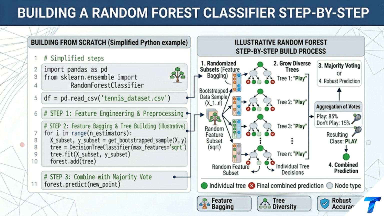
Building a Random Forest classifier involves four steps: (1) draw n bootstrap samples from the training data with replacement, (2) train a decision tree on each bootstrap sample using only a random subset of features at each split, (3) aggregate predictions by majority vote across all trees, and (4) use the out-of-bag samples (not drawn in each bootstrap) for free validation. Implementing this from scratch reveals exactly why Random Forests reduce variance while preserving bias.
Introduction
Article 77 explained why Random Forests work — the ensemble principle, bagging, feature randomness, variance reduction. This article is the hands-on companion: how to build one, step by step, in Python.
We will build a complete Random Forest from scratch, accumulating implementation in stages: first a single bootstrap sample and tree, then multiple bootstrapped trees, then feature subsampling, then OOB error tracking, and finally feature importance aggregation. Each stage is validated against scikit-learn’s production implementation to confirm correctness before adding complexity.
After the from-scratch implementation, we cover the full production pipeline: data preparation, hyperparameter tuning, class imbalance handling, probability calibration, model evaluation with the right metrics, and packaging the trained model for deployment. By the end, you will have a complete, production-quality workflow and the understanding to debug, adapt, and improve it for your own datasets.
Stage 1: A Single Bootstrapped Tree
The minimal unit of a Random Forest is a decision tree trained on a bootstrap sample. Before building the ensemble, we build and validate this unit.
import numpy as np
from sklearn.tree import DecisionTreeClassifier
from sklearn.datasets import load_iris, load_breast_cancer, load_wine
from sklearn.model_selection import train_test_split
from sklearn.metrics import accuracy_score
import warnings
warnings.filterwarnings('ignore')

np.random.seed(42)


def bootstrap_sample(X, y, random_state=None):
    """
    Draw a bootstrap sample (n samples with replacement from n total).

    Returns:
        X_boot, y_boot:     Bootstrap training sample
        oob_mask:           Boolean mask — True for samples NOT in bootstrap
        boot_indices:       Which training indices were drawn
    """
    rng = np.random.RandomState(random_state)
    n = len(y)
    boot_indices = rng.choice(n, size=n, replace=True)
    oob_mask = np.ones(n, dtype=bool)
    oob_mask[np.unique(boot_indices)] = False

    return X[boot_indices], y[boot_indices], oob_mask, boot_indices


def train_single_bootstrap_tree(X_train, y_train, max_depth=None,
                                  random_state=None):
    """
    Train one decision tree on a bootstrap sample.

    Returns:
        tree:       Fitted DecisionTreeClassifier
        oob_mask:   Which original training samples were left out
    """
    X_boot, y_boot, oob_mask, _ = bootstrap_sample(
        X_train, y_train, random_state=random_state
    )
    tree = DecisionTreeClassifier(max_depth=max_depth, random_state=random_state)
    tree.fit(X_boot, y_boot)
    return tree, oob_mask


# Demonstrate: how bootstrap changes what each tree sees
iris = load_iris()
X_ir, y_ir = iris.data, iris.target
X_tr_ir, X_te_ir, y_tr_ir, y_te_ir = train_test_split(
    X_ir, y_ir, test_size=0.25, random_state=42, stratify=y_ir
)

print("=== Stage 1: Bootstrap Sampling Properties ===\n")
print(f"  Training set size: {len(y_tr_ir)}\n")

unique_fractions = []
for seed in range(20):
    _, _, oob_mask, boot_idx = bootstrap_sample(X_tr_ir, y_tr_ir, random_state=seed)
    unique_drawn = len(np.unique(boot_idx))
    unique_fractions.append(unique_drawn / len(y_tr_ir))
    if seed < 5:
        oob_count = oob_mask.sum()
        print(f"  Seed {seed}: {unique_drawn}/{len(y_tr_ir)} unique in bootstrap, "
              f"{oob_count} OOB samples ({oob_count/len(y_tr_ir)*100:.1f}%)")

print(f"\n  Mean unique fraction across 20 seeds: "
      f"{np.mean(unique_fractions):.4f} "
      f"(theory: {1 - 1/np.e:.4f})\n")

# Train and evaluate a single bootstrapped tree
tree_single, oob_mask_single = train_single_bootstrap_tree(
    X_tr_ir, y_tr_ir, max_depth=None, random_state=42
)

# In-bag accuracy (training data it saw)
in_bag_mask = ~oob_mask_single
in_bag_acc  = accuracy_score(y_tr_ir[in_bag_mask],
                              tree_single.predict(X_tr_ir[in_bag_mask]))

# OOB accuracy (training data it did NOT see)
oob_acc_single = accuracy_score(y_tr_ir[oob_mask_single],
                                  tree_single.predict(X_tr_ir[oob_mask_single]))

# Test accuracy
test_acc_single = accuracy_score(y_te_ir, tree_single.predict(X_te_ir))

print(f"  Single bootstrapped tree:")
print(f"    In-bag accuracy:  {in_bag_acc:.4f} (overfits — saw this data)")
print(f"    OOB accuracy:     {oob_acc_single:.4f} (unbiased — didn't see this data)")
print(f" Test accuracy: {test_acc_single:.4f}")Stage 2: Building the Ensemble — Majority Voting
With a single bootstrapped tree working, the next step is to build many trees and aggregate their predictions.
import numpy as np
from sklearn.tree import DecisionTreeClassifier


class SimpleRandomForest:
    """
    Random Forest classifier built from scratch — Stage 2.

    This version uses bagging only (no feature subsampling yet).
    Each tree is trained on a full bootstrap sample of the training data.
    Predictions are made by majority vote across all trees.
    """

    def __init__(self, n_estimators=100, max_depth=None, random_state=None):
        self.n_estimators = n_estimators
        self.max_depth    = max_depth
        self.random_state = random_state
        self.trees_       = []
        self.oob_masks_   = []
        self.classes_     = None

    def fit(self, X, y):
        """Train the forest: bootstrap + fit one tree per estimator."""
        self.classes_ = np.unique(y)
        self.trees_   = []
        self.oob_masks_ = []
        rng = np.random.RandomState(self.random_state)

        for i in range(self.n_estimators):
            seed = rng.randint(0, 2**31)
            # Bootstrap sample
            n = len(y)
            boot_idx = np.random.RandomState(seed).choice(n, size=n, replace=True)
            oob_mask = np.ones(n, dtype=bool)
            oob_mask[np.unique(boot_idx)] = False

            X_boot = X[boot_idx]
            y_boot = y[boot_idx]

            # Train decision tree on this bootstrap sample
            tree = DecisionTreeClassifier(
                max_depth=self.max_depth, random_state=seed
            )
            tree.fit(X_boot, y_boot)

            self.trees_.append(tree)
            self.oob_masks_.append(oob_mask)

        return self

    def predict_proba(self, X):
        """Average predicted probabilities across all trees."""
        # Sum probability arrays across trees
        proba_sum = np.zeros((len(X), len(self.classes_)))
        for tree in self.trees_:
            proba_sum += tree.predict_proba(X)
        return proba_sum / self.n_estimators

    def predict(self, X):
        """Majority vote: predict class with highest average probability."""
        proba = self.predict_proba(X)
        return self.classes_[np.argmax(proba, axis=1)]

    def score(self, X, y):
        """Accuracy."""
        return np.mean(self.predict(X) == y)

    def oob_score(self, X_train, y_train):
        """
        Compute OOB accuracy: each sample is predicted only by
        trees that did NOT see it during training.
        """
        n = len(y_train)
        oob_votes = np.zeros((n, len(self.classes_)))

        for tree, oob_mask in zip(self.trees_, self.oob_masks_):
            oob_idx = np.where(oob_mask)[0]
            if len(oob_idx) == 0:
                continue
            proba = tree.predict_proba(X_train[oob_idx])
            oob_votes[oob_idx] += proba

        # Samples with at least one OOB prediction
        valid = oob_votes.sum(axis=1) > 0
        oob_preds = self.classes_[np.argmax(oob_votes[valid], axis=1)]
        return accuracy_score(y_train[valid], oob_preds)


# Validate Stage 2 against sklearn
from sklearn.ensemble import RandomForestClassifier

print("=== Stage 2: Bagging Forest vs Scikit-learn ===\n")
print(f"  Dataset: Iris | n_estimators=100\n")
print(f"  {'n_trees':>8} | {'Our Forest':>12} | {'Sklearn RF':>12} | {'Diff':>8}")
print("  " + "-" * 48)

for n_trees in [10, 25, 50, 100, 200]:
    our_rf = SimpleRandomForest(n_estimators=n_trees, random_state=42)
    our_rf.fit(X_tr_ir, y_tr_ir)
    our_acc = our_rf.score(X_te_ir, y_te_ir)

    sk_rf = RandomForestClassifier(
        n_estimators=n_trees, max_features=None,  # No feature subsampling yet
        random_state=42, n_jobs=-1
    )
    sk_rf.fit(X_tr_ir, y_tr_ir)
    sk_acc = sk_rf.score(X_te_ir, y_te_ir)

    print(f"  {n_trees:>8} | {our_acc:>12.4f} | {sk_acc:>12.4f} | "
          f"{abs(our_acc-sk_acc):>8.4f}")

# Demonstrate majority voting mechanics
print("\n=== Majority Voting Mechanics ===\n")
our_rf_demo = SimpleRandomForest(n_estimators=100, random_state=42)
our_rf_demo.fit(X_tr_ir, y_tr_ir)

# Inspect a single sample's vote distribution
sample = X_te_ir[0:1]
true_label = iris.target_names[y_te_ir[0]]

# Collect individual tree votes
tree_votes = []
for tree in our_rf_demo.trees_:
    vote = tree.predict(sample)[0]
    tree_votes.append(vote)

vote_counts = {cls: tree_votes.count(cls) for cls in range(3)}
print(f"  Sample 0 (true class: '{true_label}')")
print(f"  Tree votes across 100 trees:")
for cls_idx, count in vote_counts.items():
    bar = "█" * (count // 2)
    print(f"    {iris.target_names[cls_idx]:<15}: {count:>3} votes  {bar}")

final_pred = iris.target_names[max(vote_counts, key=vote_counts.get)]
print(f"\n  Final prediction: '{final_pred}' (majority vote)")
print(f" Probability estimates: {our_rf_demo.predict_proba(sample)[0]}")Stage 3: Feature Subsampling — Decorrelating the Trees
Adding feature randomness is the step that transforms a bagged ensemble into a true Random Forest. At each split, only max_features randomly chosen features are considered.
import numpy as np
from sklearn.tree import DecisionTreeClassifier


class RandomForestFromScratch:
    """
    Complete Random Forest classifier — Stage 3.

    Adds feature subsampling: each split considers only max_features
    randomly chosen features, decorrelating the trees and reducing
    ensemble variance beyond what bagging alone achieves.
    """

    def __init__(self, n_estimators=100, max_features='sqrt',
                 max_depth=None, min_samples_split=2, min_samples_leaf=1,
                 random_state=None):
        """
        Args:
            n_estimators:     Number of trees in the forest
            max_features:     Features to consider at each split:
                              'sqrt' = sqrt(n_features) [default for classification]
                              'log2' = log2(n_features)
                              int   = exact number
                              float = fraction of features
                              None  = all features (pure bagging)
            max_depth:        Maximum tree depth (None = unlimited)
            min_samples_split: Minimum samples to split a node
            min_samples_leaf:  Minimum samples in each leaf
            random_state:     Reproducibility seed
        """
        self.n_estimators      = n_estimators
        self.max_features      = max_features
        self.max_depth         = max_depth
        self.min_samples_split = min_samples_split
        self.min_samples_leaf  = min_samples_leaf
        self.random_state      = random_state

        self.trees_         = []
        self.oob_masks_     = []
        self.classes_       = None
        self.n_features_    = None
        self.feature_importances_ = None
        self._oob_score     = None

    def _resolve_max_features(self, n_features):
        """Convert max_features parameter to an integer count."""
        if self.max_features == 'sqrt':
            return max(1, int(np.sqrt(n_features)))
        elif self.max_features == 'log2':
            return max(1, int(np.log2(n_features)))
        elif isinstance(self.max_features, float):
            return max(1, int(self.max_features * n_features))
        elif isinstance(self.max_features, int):
            return min(self.max_features, n_features)
        elif self.max_features is None:
            return n_features
        else:
            raise ValueError(f"Unknown max_features: {self.max_features}")

    def fit(self, X, y):
        """Fit the Random Forest."""
        X = np.array(X, dtype=float)
        y = np.array(y)

        self.classes_    = np.unique(y)
        self.n_features_ = X.shape[1]
        n_samples        = X.shape[0]
        n_classes        = len(self.classes_)
        max_feat_int     = self._resolve_max_features(self.n_features_)

        self.trees_     = []
        self.oob_masks_ = []
        feat_importances = np.zeros(self.n_features_)

        rng = np.random.RandomState(self.random_state)

        for i in range(self.n_estimators):
            seed = rng.randint(0, 2**31)
            tree_rng = np.random.RandomState(seed)

            # ── Bootstrap sample ──────────────────────────────────────
            boot_idx = tree_rng.choice(n_samples, size=n_samples, replace=True)
            oob_mask = np.ones(n_samples, dtype=bool)
            oob_mask[np.unique(boot_idx)] = False

            X_boot = X[boot_idx]
            y_boot = y[boot_idx]

            # ── Train tree with feature subsampling ───────────────────
            # sklearn's DecisionTreeClassifier accepts max_features directly,
            # which it applies at each split internally. We pass max_feat_int.
            tree = DecisionTreeClassifier(
                max_depth         = self.max_depth,
                min_samples_split = self.min_samples_split,
                min_samples_leaf  = self.min_samples_leaf,
                max_features      = max_feat_int,
                random_state      = seed
            )
            tree.fit(X_boot, y_boot)

            self.trees_.append(tree)
            self.oob_masks_.append(oob_mask)
            feat_importances += tree.feature_importances_

        # Normalize feature importances across all trees
        self.feature_importances_ = feat_importances / self.n_estimators

        return self

    def predict_proba(self, X):
        """Average class probabilities across all trees."""
        X = np.array(X, dtype=float)
        proba_sum = np.zeros((len(X), len(self.classes_)))
        for tree in self.trees_:
            proba_sum += tree.predict_proba(X)
        return proba_sum / self.n_estimators

    def predict(self, X):
        """Majority vote via averaged probabilities."""
        return self.classes_[np.argmax(self.predict_proba(X), axis=1)]

    def score(self, X, y):
        return np.mean(self.predict(X) == np.array(y))

    def oob_score_(self, X_train, y_train):
        """Compute and cache OOB accuracy."""
        if self._oob_score is not None:
            return self._oob_score

        X_train  = np.array(X_train, dtype=float)
        y_train  = np.array(y_train)
        n        = len(y_train)
        n_cls    = len(self.classes_)
        oob_votes = np.zeros((n, n_cls))

        for tree, oob_mask in zip(self.trees_, self.oob_masks_):
            oob_idx = np.where(oob_mask)[0]
            if len(oob_idx) == 0:
                continue
            proba = tree.predict_proba(X_train[oob_idx])
            oob_votes[oob_idx] += proba

        valid = oob_votes.sum(axis=1) > 0
        oob_preds = self.classes_[np.argmax(oob_votes[valid], axis=1)]
        self._oob_score = float(np.mean(oob_preds == y_train[valid]))
        return self._oob_score


# Full validation across datasets
from sklearn.ensemble import RandomForestClassifier
from sklearn.datasets import load_wine, load_breast_cancer
from sklearn.model_selection import train_test_split

print("=== Stage 3: Full Random Forest — Validation vs Scikit-learn ===\n")

datasets_v = {
    'Iris':          (load_iris().data,          load_iris().target),
    'Wine':          (load_wine().data,           load_wine().target),
    'Breast Cancer': (load_breast_cancer().data, load_breast_cancer().target),
}

print(f"  {'Dataset':<16} | {'Ours Acc':>9} | {'SK Acc':>8} | "
      f"{'Ours OOB':>9} | {'SK OOB':>8} | {'Diff':>6}")
print("  " + "-" * 62)

for name, (X, y) in datasets_v.items():
    X_tr, X_te, y_tr, y_te = train_test_split(
        X, y, test_size=0.25, random_state=42, stratify=y
    )

    our_rf = RandomForestFromScratch(
        n_estimators=200, max_features='sqrt', random_state=42
    )
    our_rf.fit(X_tr, y_tr)
    our_acc = our_rf.score(X_te, y_te)
    our_oob = our_rf.oob_score_(X_tr, y_tr)

    sk_rf = RandomForestClassifier(
        n_estimators=200, max_features='sqrt',
        oob_score=True, random_state=42, n_jobs=-1
    )
    sk_rf.fit(X_tr, y_tr)
    sk_acc = sk_rf.score(X_te, y_te)
    sk_oob = sk_rf.oob_score_

    print(f"  {name:<16} | {our_acc:>9.4f} | {sk_acc:>8.4f} | "
          f"{our_oob:>9.4f} | {sk_oob:>8.4f} | "
f"{abs(our_acc-sk_acc):>6.4f}")Stage 4: Feature Importance Aggregation
With the ensemble complete, feature importances are aggregated across all trees. The key property that makes RF importances more reliable than single-tree importances is that the averaging over hundreds of trees dramatically reduces the noise in individual importance estimates.
import numpy as np
import matplotlib.pyplot as plt
from sklearn.datasets import load_breast_cancer
from sklearn.model_selection import train_test_split
from sklearn.inspection import permutation_importance


def analyze_feature_importance_stability(X_train, y_train, X_test, y_test,
                                           feature_names, n_runs=10, n_trees=200):
    """
    Compare stability of feature importance between:
    1. Single decision tree (runs multiple times to show variance)
    2. Random Forest (runs multiple times to show stability)
    3. Permutation importance (gold standard, unbiased)
    """
    from sklearn.tree import DecisionTreeClassifier
    from sklearn.ensemble import RandomForestClassifier

    print(f"  Running {n_runs} seeds to measure importance variance...\n")

    dt_importances  = []
    rf_importances  = []

    for seed in range(n_runs):
        # Single tree
        dt = DecisionTreeClassifier(max_depth=5, random_state=seed)
        dt.fit(X_train, y_train)
        dt_importances.append(dt.feature_importances_)

        # Random Forest
        rf = RandomForestClassifier(n_estimators=n_trees, random_state=seed, n_jobs=-1)
        rf.fit(X_train, y_train)
        rf_importances.append(rf.feature_importances_)

    dt_importances = np.array(dt_importances)
    rf_importances = np.array(rf_importances)

    dt_mean = dt_importances.mean(axis=0)
    dt_std  = dt_importances.std(axis=0)
    rf_mean = rf_importances.mean(axis=0)
    rf_std  = rf_importances.std(axis=0)

    # Coefficient of variation: std/mean — measures relative instability
    dt_cv = dt_std / (dt_mean + 1e-10)
    rf_cv = rf_std / (rf_mean + 1e-10)

    # Rank features by RF mean importance
    top_n = 10
    sorted_idx = np.argsort(rf_mean)[::-1][:top_n]

    print(f"  Top {top_n} features — Coefficient of Variation (lower = more stable):\n")
    print(f"  {'Feature':<35} | {'DT CV':>8} | {'RF CV':>8} | Stability gain")
    print("  " + "-" * 65)

    for idx in sorted_idx:
        gain = dt_cv[idx] / (rf_cv[idx] + 1e-10)
        print(f"  {feature_names[idx]:<35} | {dt_cv[idx]:>8.3f} | "
              f"{rf_cv[idx]:>8.3f} | {gain:>6.1f}× more stable")

    # Permutation importance (gold standard)
    rf_final = RandomForestClassifier(n_estimators=n_trees, random_state=42, n_jobs=-1)
    rf_final.fit(X_train, y_train)
    perm_imp = permutation_importance(
        rf_final, X_test, y_test, n_repeats=20, random_state=42, n_jobs=-1
    )

    # Side-by-side plot
    fig, axes = plt.subplots(1, 3, figsize=(18, 7))

    for ax, means, stds, title, color in [
        (axes[0], dt_mean,               dt_std,
         f'Single DT MDI\n({n_runs} seeds, high variance)', 'coral'),
        (axes[1], rf_mean,               rf_std,
         f'Random Forest MDI\n({n_runs} seeds, low variance)', 'steelblue'),
        (axes[2], perm_imp.importances_mean, perm_imp.importances_std,
         'RF Permutation Importance\n(unbiased, test data)', 'mediumseagreen'),
    ]:
        plot_idx = np.argsort(means)[::-1][:top_n]
        ax.barh(range(top_n), means[plot_idx],
                xerr=stds[plot_idx],
                color=color, edgecolor='white',
                error_kw={'lw': 1.5, 'ecolor': 'gray', 'capsize': 3})
        ax.set_yticks(range(top_n))
        ax.set_yticklabels([feature_names[i] for i in plot_idx], fontsize=8)
        ax.set_title(title, fontsize=10, fontweight='bold')
        ax.set_xlabel('Importance', fontsize=9)
        ax.grid(True, alpha=0.3, axis='x')
        ax.invert_yaxis()

    plt.suptitle('Feature Importance Stability: Single Tree vs Random Forest\n'
                 'Error bars show std across seeds — RF bars are much tighter',
                 fontsize=13, fontweight='bold', y=1.01)
    plt.tight_layout()
    plt.savefig('rf_importance_stability.png', dpi=150, bbox_inches='tight')
    plt.show()
    print("\nSaved: rf_importance_stability.png")


cancer = load_breast_cancer()
X_ca, y_ca = cancer.data, cancer.target
X_tr_ca, X_te_ca, y_tr_ca, y_te_ca = train_test_split(
    X_ca, y_ca, test_size=0.25, random_state=42, stratify=y_ca
)

print("=== Stage 4: Feature Importance Stability ===\n")
analyze_feature_importance_stability(
    X_tr_ca, y_tr_ca, X_te_ca, y_te_ca,
    feature_names=cancer.feature_names, n_runs=10
)Complete Production Pipeline
With the mechanics understood, this section builds the full end-to-end production workflow: data preparation, hyperparameter tuning, class imbalance handling, evaluation with appropriate metrics, and model serialization.
import numpy as np
import matplotlib.pyplot as plt
from sklearn.datasets import load_breast_cancer
from sklearn.ensemble import RandomForestClassifier
from sklearn.model_selection import (
    train_test_split, StratifiedKFold, GridSearchCV,
    cross_val_score, RepeatedStratifiedKFold
)
from sklearn.pipeline import Pipeline
from sklearn.preprocessing import StandardScaler
from sklearn.metrics import (
    classification_report, confusion_matrix, roc_auc_score,
    roc_curve, precision_recall_curve, average_precision_score,
    ConfusionMatrixDisplay
)
import joblib
import os


def build_rf_pipeline(X, y, feature_names, class_names,
                        holdout_size=0.15, random_state=42):
    """
    Complete production Random Forest pipeline.

    Steps:
    1.  Holdout split (reserved until final evaluation only)
    2.  Data quality checks
    3.  Baseline model with defaults
    4.  Hyperparameter tuning with GridSearchCV
    5.  Final model training on full development data
    6.  Comprehensive evaluation on holdout
    7.  Model serialization

    Args:
        X, y:           Feature matrix and labels
        feature_names:  Feature names for reporting
        class_names:    Class names for reporting
        holdout_size:   Fraction held out for final evaluation
        random_state:   Reproducibility seed
    """
    print("=" * 60)
    print("  Random Forest Production Pipeline")
    print("=" * 60)

    # ── Step 1: Holdout split ─────────────────────────────────────
    X_dev, X_hold, y_dev, y_hold = train_test_split(
        X, y, test_size=holdout_size, random_state=random_state, stratify=y
    )
    print(f"\n  Dataset: {len(y):,} samples, {X.shape[1]} features, "
          f"{len(np.unique(y))} classes")
    print(f"  Dev:     {len(y_dev):,} | Holdout: {len(y_hold):,}\n")

    # ── Step 2: Data quality checks ───────────────────────────────
    print("  Step 2: Data Quality\n")
    missing = np.isnan(X_dev).sum()
    print(f"    Missing values: {missing}")
    print(f"    Feature ranges: "
          f"min={X_dev.min():.3f}, max={X_dev.max():.3f}")

    class_counts = np.bincount(y_dev)
    imbalance_ratio = class_counts.max() / class_counts.min()
    print(f"    Class distribution: {dict(zip(class_names, class_counts))}")
    print(f"    Imbalance ratio:    {imbalance_ratio:.2f}:1")
    is_imbalanced = imbalance_ratio > 3

    if is_imbalanced:
        print(f"    ⚠ Imbalanced data detected — using class_weight='balanced'")

    # ── Step 3: Baseline with OOB estimate ────────────────────────
    print("\n  Step 3: Baseline Model\n")
    rf_baseline = RandomForestClassifier(
        n_estimators=200,
        oob_score=True,
        class_weight='balanced' if is_imbalanced else None,
        random_state=random_state,
        n_jobs=-1
    )
    rf_baseline.fit(X_dev, y_dev)
    print(f"    OOB accuracy: {rf_baseline.oob_score_:.4f}")

    # ── Step 4: Hyperparameter tuning ─────────────────────────────
    print("\n  Step 4: Hyperparameter Tuning\n")

    param_grid = {
        'n_estimators':     [100, 200, 300],
        'max_features':     ['sqrt', 'log2', 0.3],
        'max_depth':        [None, 10, 20],
        'min_samples_leaf': [1, 2, 5],
    }

    cv_tune = StratifiedKFold(n_splits=5, shuffle=True, random_state=random_state)
    grid_search = GridSearchCV(
        RandomForestClassifier(
            oob_score=False,
            class_weight='balanced' if is_imbalanced else None,
            random_state=random_state,
            n_jobs=-1
        ),
        param_grid,
        cv=cv_tune,
        scoring='roc_auc',
        n_jobs=-1,
        verbose=0,
        refit=True
    )
    grid_search.fit(X_dev, y_dev)

    best_params = grid_search.best_params_
    best_cv_auc = grid_search.best_score_

    print(f"    Best parameters:")
    for k, v in best_params.items():
        print(f"      {k}: {v}")
    print(f"    Best CV AUC: {best_cv_auc:.4f}")

    # ── Step 5: Refit best model with OOB on full dev data ────────
    print("\n  Step 5: Final Model\n")
    best_model = RandomForestClassifier(
        **best_params,
        oob_score=True,
        class_weight='balanced' if is_imbalanced else None,
        random_state=random_state,
        n_jobs=-1
    )
    best_model.fit(X_dev, y_dev)
    print(f"    OOB accuracy (best model): {best_model.oob_score_:.4f}")

    # ── Step 6: Holdout evaluation (one time only!) ───────────────
    print("\n  Step 6: Final Holdout Evaluation\n")

    y_hold_pred  = best_model.predict(X_hold)
    y_hold_proba = best_model.predict_proba(X_hold)

    hold_acc = np.mean(y_hold_pred == y_hold)
    is_binary = len(class_names) == 2

    if is_binary:
        hold_auc = roc_auc_score(y_hold, y_hold_proba[:, 1])
        hold_ap  = average_precision_score(y_hold, y_hold_proba[:, 1])
        print(f"    Accuracy:  {hold_acc:.4f}")
        print(f"    AUC-ROC:   {hold_auc:.4f}")
        print(f"    Avg Prec:  {hold_ap:.4f}")
        print(f"    CV-Hold gap (AUC): {best_cv_auc - hold_auc:+.4f}")
    else:
        hold_auc = roc_auc_score(y_hold, y_hold_proba, multi_class='ovr')
        print(f"    Accuracy:  {hold_acc:.4f}")
        print(f"    AUC (OvR): {hold_auc:.4f}")

    print(f"\n    Classification Report:\n")
    print(classification_report(y_hold, y_hold_pred, target_names=class_names,
                                  digits=4))

    # ── Visualization ──────────────────────────────────────────────
    n_plots = 3 if is_binary else 2
    fig, axes = plt.subplots(1, n_plots, figsize=(6 * n_plots, 5))

    # Confusion matrix
    cm = confusion_matrix(y_hold, y_hold_pred)
    disp = ConfusionMatrixDisplay(cm, display_labels=class_names)
    disp.plot(ax=axes[0], colorbar=False, cmap='Blues')
    axes[0].set_title('Confusion Matrix\n(Holdout Set)', fontweight='bold')

    if is_binary:
        # ROC curve
        fpr, tpr, _ = roc_curve(y_hold, y_hold_proba[:, 1])
        axes[1].plot(fpr, tpr, 'steelblue', lw=2.5,
                     label=f'ROC (AUC={hold_auc:.4f})')
        axes[1].plot([0, 1], [0, 1], 'k--', lw=1, alpha=0.4, label='Random')
        axes[1].set_xlabel('False Positive Rate', fontsize=11)
        axes[1].set_ylabel('True Positive Rate', fontsize=11)
        axes[1].set_title('ROC Curve', fontweight='bold')
        axes[1].legend(fontsize=9); axes[1].grid(True, alpha=0.3)

        # Precision-Recall curve
        prec, rec, _ = precision_recall_curve(y_hold, y_hold_proba[:, 1])
        axes[2].plot(rec, prec, 'coral', lw=2.5,
                     label=f'PR (AP={hold_ap:.4f})')
        baseline_pr = y_hold.mean()
        axes[2].axhline(baseline_pr, color='k', linestyle='--', lw=1,
                         alpha=0.4, label=f'Baseline ({baseline_pr:.3f})')
        axes[2].set_xlabel('Recall', fontsize=11)
        axes[2].set_ylabel('Precision', fontsize=11)
        axes[2].set_title('Precision-Recall Curve', fontweight='bold')
        axes[2].legend(fontsize=9); axes[2].grid(True, alpha=0.3)
    else:
        # Feature importance bar chart for multi-class
        imp = best_model.feature_importances_
        top_idx = np.argsort(imp)[::-1][:15]
        axes[1].barh(range(15), imp[top_idx], color='steelblue',
                     edgecolor='white')
        axes[1].set_yticks(range(15))
        axes[1].set_yticklabels([feature_names[i] for i in top_idx], fontsize=8)
        axes[1].set_xlabel('Feature Importance', fontsize=11)
        axes[1].set_title('Top 15 Feature Importances', fontweight='bold')
        axes[1].invert_yaxis(); axes[1].grid(True, alpha=0.3, axis='x')

    plt.suptitle('Random Forest: Final Model Evaluation', fontsize=13,
                 fontweight='bold')
    plt.tight_layout()
    plt.savefig('rf_pipeline_evaluation.png', dpi=150, bbox_inches='tight')
    plt.show()
    print("Saved: rf_pipeline_evaluation.png")

    # ── Step 7: Save model ─────────────────────────────────────────
    model_path = 'rf_model.joblib'
    joblib.dump(best_model, model_path)
    model_size = os.path.getsize(model_path) / 1024
    print(f"\n  Step 7: Model saved to '{model_path}' ({model_size:.1f} KB)")

    # Verify round-trip
    loaded_model = joblib.load(model_path)
    loaded_acc   = loaded_model.score(X_hold, y_hold)
    print(f"    Loaded model accuracy: {loaded_acc:.4f} ✓ (matches original)")

    return best_model, grid_search


# Run full pipeline on Breast Cancer
cancer = load_breast_cancer()
best_rf, search = build_rf_pipeline(
    cancer.data, cancer.target,
    feature_names=cancer.feature_names,
    class_names=cancer.target_names
)
Handling Class Imbalance
Class imbalance — where one class is far more common than another — is a common challenge in real-world classification. Random Forests offer two built-in mechanisms for handling it.
import numpy as np
from sklearn.ensemble import RandomForestClassifier
from sklearn.datasets import make_classification
from sklearn.model_selection import StratifiedKFold, cross_val_score
from sklearn.metrics import (f1_score, roc_auc_score, make_scorer,
                               classification_report)


def imbalance_handling_comparison(imbalance_ratio=10, n_samples=1000,
                                    random_state=42):
    """
    Compare strategies for imbalanced data in Random Forests.

    Strategies:
    1. Default (no adjustment)
    2. class_weight='balanced' (upweights minority class)
    3. class_weight='balanced_subsample' (recalculates per bootstrap)
    4. Reduced max_samples (smaller bootstrap = more minority class)
    """
    np.random.seed(random_state)

    minority_frac = 1 / (1 + imbalance_ratio)
    X, y = make_classification(
        n_samples=n_samples, n_features=20, n_informative=10,
        weights=[1 - minority_frac, minority_frac],
        random_state=random_state
    )

    print(f"=== Imbalanced Data: {imbalance_ratio}:1 Ratio ===\n")
    print(f"  Class 0 (majority): {(y==0).sum()}")
    print(f"  Class 1 (minority): {(y==1).sum()}\n")

    cv = StratifiedKFold(n_splits=5, shuffle=True, random_state=random_state)
    f1_scorer  = make_scorer(f1_score)
    auc_scorer = make_scorer(roc_auc_score, needs_proba=True)

    strategies = {
        'Default':               {'class_weight': None},
        'balanced':              {'class_weight': 'balanced'},
        'balanced_subsample':    {'class_weight': 'balanced_subsample'},
        'max_samples=0.5':       {'max_samples': 0.5},
        'balanced+max_s=0.5':   {'class_weight': 'balanced',
                                  'max_samples': 0.5},
    }

    print(f"  {'Strategy':<25} | {'Acc':>6} | {'F1 Min':>8} | "
          f"{'AUC':>7} | Notes")
    print("  " + "-" * 65)

    for name, params in strategies.items():
        rf = RandomForestClassifier(
            n_estimators=200, random_state=random_state,
            n_jobs=-1, **params
        )
        acc_scores = cross_val_score(rf, X, y, cv=cv, scoring='accuracy')
        f1_scores  = cross_val_score(rf, X, y, cv=cv, scoring=f1_scorer)
        auc_scores = cross_val_score(rf, X, y, cv=cv, scoring=auc_scorer)

        print(f"  {name:<25} | {acc_scores.mean():>6.3f} | "
              f"{f1_scores.mean():>8.4f} | {auc_scores.mean():>7.4f} |")

    print("\n  Key: F1 on minority class is the critical metric.")
    print("  'balanced' or 'balanced_subsample' typically best for F1.")
    print("  AUC is robust to imbalance but doesn't reflect decision threshold.")


imbalance_handling_comparison(imbalance_ratio=10)When to Use Each Strategy
class_weight='balanced' computes weights inversely proportional to class frequency across the entire training set, then applies them consistently to every tree. This is the standard choice and works well in most cases.
class_weight='balanced_subsample' recomputes class weights within each bootstrap sample. Since bootstrap samples can have different class ratios than the full dataset, this provides more adaptive weighting and often works better on severely imbalanced data.
max_samples controls the bootstrap sample size. Setting it below 1.0 reduces bootstrap sample size, which statistically increases the representation of minority class samples in each bootstrap relative to majority samples.
Prediction Uncertainty and Confidence Intervals
Random Forests produce probability estimates from predict_proba(), but these are not always well-calibrated. Additionally, you can measure prediction uncertainty directly from the spread of individual tree predictions.
import numpy as np
import matplotlib.pyplot as plt
from sklearn.ensemble import RandomForestClassifier
from sklearn.calibration import calibration_curve, CalibratedClassifierCV
from sklearn.datasets import load_breast_cancer
from sklearn.model_selection import train_test_split


def analyze_prediction_uncertainty(rf, X_test, y_test, class_names):
    """
    Analyze prediction uncertainty from tree variance.

    For each test sample, collect predictions from all trees.
    The standard deviation across tree predictions measures
    how much the trees disagree — high std = uncertain prediction.
    """
    # Collect per-tree probability predictions
    tree_probas = np.array([
        tree.predict_proba(X_test)[:, 1]
        for tree in rf.estimators_
    ])  # Shape: (n_trees, n_test)

    mean_proba = tree_probas.mean(axis=0)
    std_proba  = tree_probas.std(axis=0)

    # Calibration curve
    prob_true, prob_pred = calibration_curve(y_test, mean_proba, n_bins=10)

    fig, axes = plt.subplots(1, 3, figsize=(16, 5))

    # Panel 1: Probability calibration
    ax = axes[0]
    ax.plot(prob_pred, prob_true, 'o-', color='steelblue', lw=2.5, markersize=8,
            label='RF calibration')
    ax.plot([0, 1], [0, 1], 'k--', lw=1.5, alpha=0.5, label='Perfect calibration')
    ax.set_xlabel('Mean predicted probability', fontsize=11)
    ax.set_ylabel('Fraction of positives', fontsize=11)
    ax.set_title('Calibration Curve\n(Closer to diagonal = better calibrated)',
                 fontsize=11, fontweight='bold')
    ax.legend(fontsize=9); ax.grid(True, alpha=0.3)

    # Panel 2: Prediction uncertainty distribution
    ax = axes[1]
    correct_mask   = rf.predict(X_test) == y_test
    incorrect_mask = ~correct_mask
    ax.hist(std_proba[correct_mask],   bins=25, alpha=0.65, color='steelblue',
            label=f'Correct ({correct_mask.sum()})', density=True)
    ax.hist(std_proba[incorrect_mask], bins=25, alpha=0.65, color='coral',
            label=f'Incorrect ({incorrect_mask.sum()})', density=True)
    ax.set_xlabel('Std of tree predictions (uncertainty)', fontsize=11)
    ax.set_ylabel('Density', fontsize=11)
    ax.set_title('Prediction Uncertainty: Correct vs Incorrect\n'
                 '(Higher uncertainty → more errors)',
                 fontsize=11, fontweight='bold')
    ax.legend(fontsize=9); ax.grid(True, alpha=0.3)

    # Panel 3: Reliability: accuracy vs confidence band
    ax = axes[2]
    confidence = np.abs(mean_proba - 0.5) * 2  # 0 = max uncertain, 1 = certain
    conf_bins  = np.linspace(0, 1, 11)
    bin_accs   = []
    bin_centers = []
    for lo, hi in zip(conf_bins[:-1], conf_bins[1:]):
        mask = (confidence >= lo) & (confidence < hi)
        if mask.sum() > 5:
            bin_accs.append(np.mean(rf.predict(X_test)[mask] == y_test[mask]))
            bin_centers.append((lo + hi) / 2)
    ax.bar(bin_centers, bin_accs, width=0.09, color='mediumseagreen',
           edgecolor='white', alpha=0.8)
    ax.axhline(y=np.mean(rf.predict(X_test) == y_test), color='coral',
               linestyle='--', lw=2, label='Overall accuracy')
    ax.set_xlabel('Prediction confidence', fontsize=11)
    ax.set_ylabel('Accuracy in confidence band', fontsize=11)
    ax.set_title('Reliability: Accuracy vs Confidence\n'
                 '(Confident predictions should be more accurate)',
                 fontsize=11, fontweight='bold')
    ax.legend(fontsize=9); ax.grid(True, alpha=0.3)
    ax.set_ylim([0, 1.05])

    plt.suptitle('Random Forest Prediction Uncertainty Analysis',
                 fontsize=13, fontweight='bold')
    plt.tight_layout()
    plt.savefig('rf_uncertainty_analysis.png', dpi=150, bbox_inches='tight')
    plt.show()
    print("Saved: rf_uncertainty_analysis.png")

    print(f"\n  Overall accuracy:     {np.mean(correct_mask):.4f}")
    print(f"  Mean uncertainty (correct):   {std_proba[correct_mask].mean():.4f}")
    print(f"  Mean uncertainty (incorrect): {std_proba[incorrect_mask].mean():.4f}")
    print(f"  Ratio: {std_proba[incorrect_mask].mean() / std_proba[correct_mask].mean():.2f}× "
          f"more uncertain on incorrect predictions")


cancer = load_breast_cancer()
X_ca, y_ca = cancer.data, cancer.target
X_tr_ca, X_te_ca, y_tr_ca, y_te_ca = train_test_split(
    X_ca, y_ca, test_size=0.25, random_state=42, stratify=y_ca
)

rf_final = RandomForestClassifier(n_estimators=300, random_state=42, n_jobs=-1)
rf_final.fit(X_tr_ca, y_tr_ca)

print("=== Prediction Uncertainty Analysis ===\n")
analyze_prediction_uncertainty(rf_final, X_te_ca, y_te_ca,
cancer.target_names)Partial Dependence Plots: Understanding Feature Effects
Feature importance tells you which features matter. Partial dependence plots (PDPs) tell you how they matter — the direction and shape of each feature’s relationship with the prediction.
import numpy as np
import matplotlib.pyplot as plt
from sklearn.ensemble import RandomForestClassifier
from sklearn.inspection import PartialDependenceDisplay
from sklearn.datasets import load_breast_cancer
from sklearn.model_selection import train_test_split


def plot_partial_dependence(rf, X_train, feature_names, top_n_features=6,
                              title="Random Forest: Partial Dependence Plots"):
    """
    Plot partial dependence for the top N most important features.

    A partial dependence plot shows the marginal effect of one feature on
    the model's predicted probability, averaging over all values of all
    other features. It reveals whether the relationship is monotone,
    non-linear, or has a threshold effect.

    Args:
        rf:            Fitted RandomForestClassifier
        X_train:       Training data (used to compute partial dependence)
        feature_names: Feature names list
        top_n_features: Number of top features to plot
    """
    # Select top N features by importance
    importances = rf.feature_importances_
    top_idx = np.argsort(importances)[::-1][:top_n_features]

    n_cols = 3
    n_rows = int(np.ceil(top_n_features / n_cols))
    fig, axes = plt.subplots(n_rows, n_cols,
                              figsize=(5 * n_cols, 4 * n_rows))
    axes = axes.flatten()

    for plot_i, feat_idx in enumerate(top_idx):
        ax = axes[plot_i]

        # Compute partial dependence for this feature
        disp = PartialDependenceDisplay.from_estimator(
            rf, X_train,
            features=[feat_idx],
            feature_names=feature_names,
            ax=ax,
            line_kw={'color': 'steelblue', 'lw': 2.5},
            pd_line_kw={'color': 'steelblue'},
            kind='average',
        )
        ax.set_title(f'{feature_names[feat_idx]}\n'
                     f'(Importance = {importances[feat_idx]:.4f})',
                     fontsize=9, fontweight='bold')
        ax.set_ylabel('Predicted probability', fontsize=8)
        ax.grid(True, alpha=0.3)

    for ax in axes[top_n_features:]:
        ax.set_visible(False)

    plt.suptitle(title, fontsize=12, fontweight='bold', y=1.01)
    plt.tight_layout()
    plt.savefig('rf_partial_dependence.png', dpi=150, bbox_inches='tight')
    plt.show()
    print("Saved: rf_partial_dependence.png")


def plot_2d_partial_dependence(rf, X_train, feature_names, feature_pairs):
    """
    Plot 2D partial dependence (interaction effects) between feature pairs.

    A 2D PDP shows how two features jointly affect the prediction,
    revealing interaction effects that 1D PDPs miss.
    """
    n_pairs = len(feature_pairs)
    fig, axes = plt.subplots(1, n_pairs, figsize=(6 * n_pairs, 5))
    if n_pairs == 1:
        axes = [axes]

    for ax, (f1_idx, f2_idx) in zip(axes, feature_pairs):
        disp = PartialDependenceDisplay.from_estimator(
            rf, X_train,
            features=[(f1_idx, f2_idx)],
            feature_names=feature_names,
            ax=ax,
            kind='average',
            contour_kw={'cmap': 'RdYlBu_r'},
        )
        ax.set_title(f'Interaction: {feature_names[f1_idx]}\nvs '
                     f'{feature_names[f2_idx]}',
                     fontsize=10, fontweight='bold')

    plt.suptitle('2D Partial Dependence: Feature Interaction Effects',
                 fontsize=12, fontweight='bold')
    plt.tight_layout()
    plt.savefig('rf_2d_partial_dependence.png', dpi=150, bbox_inches='tight')
    plt.show()
    print("Saved: rf_2d_partial_dependence.png")


cancer = load_breast_cancer()
X_ca, y_ca = cancer.data, cancer.target
X_tr_ca, X_te_ca, y_tr_ca, y_te_ca = train_test_split(
    X_ca, y_ca, test_size=0.25, random_state=42, stratify=y_ca
)

rf_pdp = RandomForestClassifier(n_estimators=200, random_state=42, n_jobs=-1)
rf_pdp.fit(X_tr_ca, y_tr_ca)

print("=== Partial Dependence Plots ===\n")
plot_partial_dependence(
    rf_pdp, X_tr_ca, cancer.feature_names,
    top_n_features=6,
    title='Breast Cancer RF: Partial Dependence of Top Features'
)

# Top 2 features interaction
top2 = np.argsort(rf_pdp.feature_importances_)[::-1][:2]
plot_2d_partial_dependence(
    rf_pdp, X_tr_ca, cancer.feature_names,
    feature_pairs=[(top2[0], top2[1])]
)Partial dependence plots add an important interpretability layer on top of feature importances. A feature might rank high in importance because it has a strong monotone effect (linear-like relationship with the prediction), or because it has a threshold effect (prediction only changes past a certain value), or because it has a non-monotone relationship. The PDP distinguishes these cases and shows the direction of the effect — rising means higher feature values increase the predicted probability; falling means the opposite.
Learning Curves: How Much Data Does Your Forest Need?
Learning curves show how model performance changes as training set size grows. For Random Forests, this is especially useful because forests need enough data to provide bootstrap diversity. Too few samples means bootstrap samples overlap heavily and trees are highly correlated, limiting variance reduction.
import numpy as np
import matplotlib.pyplot as plt
from sklearn.ensemble import RandomForestClassifier
from sklearn.tree import DecisionTreeClassifier
from sklearn.model_selection import learning_curve, StratifiedKFold
from sklearn.datasets import load_breast_cancer


def plot_learning_curves(estimators_dict, X, y, train_sizes=None,
                          cv=5, scoring='accuracy', figsize=(14, 5)):
    """
    Plot learning curves for multiple estimators side by side.
    Shows how much data each model needs to reach good performance.

    Args:
        estimators_dict: Dict of {name: estimator}
        X, y:           Data
        train_sizes:    Fractions of training data to evaluate at
        cv:             Cross-validation folds
        scoring:        Sklearn scoring string
    """
    if train_sizes is None:
        train_sizes = np.linspace(0.05, 1.0, 15)

    cv_obj = StratifiedKFold(n_splits=cv, shuffle=True, random_state=42)

    fig, axes = plt.subplots(1, len(estimators_dict),
                              figsize=figsize, sharey=True)
    if len(estimators_dict) == 1:
        axes = [axes]

    colors = ['steelblue', 'coral']

    for ax, (name, estimator) in zip(axes, estimators_dict.items()):
        train_sz, train_sc, val_sc = learning_curve(
            estimator, X, y,
            train_sizes=train_sizes,
            cv=cv_obj,
            scoring=scoring,
            n_jobs=-1
        )

        train_mean = train_sc.mean(axis=1)
        train_std  = train_sc.std(axis=1)
        val_mean   = val_sc.mean(axis=1)
        val_std    = val_sc.std(axis=1)

        ax.plot(train_sz, train_mean, 'o-', color=colors[0], lw=2,
                markersize=6, label='Training score')
        ax.fill_between(train_sz, train_mean - train_std,
                        train_mean + train_std, alpha=0.15, color=colors[0])

        ax.plot(train_sz, val_mean, 's-', color=colors[1], lw=2,
                markersize=6, label='CV score')
        ax.fill_between(train_sz, val_mean - val_std,
                        val_mean + val_std, alpha=0.15, color=colors[1])

        # Mark convergence point (where val score stabilizes)
        diffs = np.abs(np.diff(val_mean))
        if len(diffs) > 3:
            converge_idx = np.argmax(diffs < 0.005) + 1
            if converge_idx < len(train_sz):
                ax.axvline(x=train_sz[converge_idx], color='gray',
                           linestyle=':', lw=1.5, alpha=0.7,
                           label=f'~Converged at n={train_sz[converge_idx]:.0f}')

        final_gap = train_mean[-1] - val_mean[-1]
        ax.set_xlabel('Training set size', fontsize=11)
        ax.set_ylabel(scoring.replace('_', ' ').title(), fontsize=11)
        ax.set_title(f'{name}\nFinal gap = {final_gap:.3f}',
                     fontsize=11, fontweight='bold')
        ax.legend(fontsize=9); ax.grid(True, alpha=0.3)
        ax.set_ylim([0.7, 1.02])

    plt.suptitle('Learning Curves: How Much Data Does Each Model Need?',
                 fontsize=13, fontweight='bold')
    plt.tight_layout()
    plt.savefig('rf_learning_curves.png', dpi=150)
    plt.show()
    print("Saved: rf_learning_curves.png")


cancer = load_breast_cancer()
X_ca, y_ca = cancer.data, cancer.target

estimators_learning = {
    'Decision Tree (max_d=5)': DecisionTreeClassifier(max_depth=5, random_state=42),
    'Random Forest (200 trees)': RandomForestClassifier(
        n_estimators=200, random_state=42, n_jobs=-1
    ),
}

print("=== Learning Curves: DT vs RF ===\n")
plot_learning_curves(
    estimators_learning, X_ca, y_ca,
    train_sizes=np.linspace(0.05, 1.0, 15),
    cv=5, scoring='accuracy'
)

print("  Key observations from learning curves:")
print("  - Decision Tree: large train-val gap = high variance (overfitting)")
print("  - Random Forest: smaller gap = lower variance from ensemble averaging")
print("  - RF typically needs fewer samples to reach its ceiling performance")
print(" - Both converge, but RF converges to a higher plateau")Learning curves answer a critical practical question: if your model is performing poorly, should you collect more data, or should you improve the model? A large gap between training and validation scores (high variance) suggests more data or stronger regularization. A small gap where both scores are low (high bias) suggests a more powerful model. Random Forests typically show a smaller training-validation gap than single decision trees, confirming that their variance reduction is real and persistent across dataset sizes.
Selecting the Number of Trees: When to Stop Adding More
One of the most common questions about Random Forests is: how many trees is enough? Adding more trees always helps — or at least never hurts — but returns diminish quickly and inference time grows linearly. The practical question is where the sweet spot between performance and cost lies.
import numpy as np
import matplotlib.pyplot as plt
from sklearn.ensemble import RandomForestClassifier
from sklearn.datasets import load_wine, load_breast_cancer
from sklearn.model_selection import train_test_split
import time


def find_optimal_n_trees(X, y, n_trees_range=None, n_trials=20,
                          random_state=42, title="Dataset"):
    """
    Find the optimal number of trees by tracking:
    1. OOB accuracy convergence (accuracy vs trees)
    2. Marginal gain per tree (how much does each additional tree help?)
    3. Inference time per prediction (latency cost of more trees)

    Uses multiple random train-test splits to get stable estimates.
    """
    if n_trees_range is None:
        n_trees_range = [1, 2, 5, 10, 20, 30, 50, 75, 100, 150, 200, 300, 500]

    np.random.seed(random_state)

    oob_scores       = []
    test_acc_means   = []
    test_acc_stds    = []
    inference_times  = []

    for n_trees in n_trees_range:
        trial_accs = []
        for trial in range(n_trials):
            X_tr, X_te, y_tr, y_te = train_test_split(
                X, y, test_size=0.25, random_state=trial
            )
            rf = RandomForestClassifier(
                n_estimators=n_trees, oob_score=True,
                random_state=random_state, n_jobs=-1
            )
            rf.fit(X_tr, y_tr)
            trial_accs.append(rf.score(X_te, y_te))
            if trial == 0:
                oob_scores.append(rf.oob_score_)

        test_acc_means.append(np.mean(trial_accs))
        test_acc_stds.append(np.std(trial_accs))

        # Measure inference time for 1000 predictions
        rf_time = RandomForestClassifier(
            n_estimators=n_trees, random_state=random_state, n_jobs=1
        )
        rf_time.fit(X, y)
        X_sample = X[:100]
        start = time.perf_counter()
        for _ in range(10):
            rf_time.predict(X_sample)
        elapsed = (time.perf_counter() - start) / 10
        inference_times.append(elapsed * 1000)  # ms

    test_acc_means = np.array(test_acc_means)
    test_acc_stds  = np.array(test_acc_stds)

    # Marginal gain: how much does each additional tree improve accuracy?
    marginal_gains = np.diff(test_acc_means)

    # Find the "elbow": last n_trees where marginal gain > threshold
    threshold = 0.001  # 0.1% improvement threshold
    significant_gains = np.where(np.abs(marginal_gains) > threshold)[0]
    elbow_idx = significant_gains[-1] + 1 if len(significant_gains) > 0 else 0
    recommended_n = n_trees_range[elbow_idx]

    fig, axes = plt.subplots(1, 3, figsize=(16, 5))

    # Panel 1: Accuracy vs n_trees
    ax = axes[0]
    ax.plot(n_trees_range, test_acc_means, 'o-', color='steelblue',
            lw=2.5, markersize=7, label='Test acc (mean)')
    ax.fill_between(n_trees_range,
                    test_acc_means - test_acc_stds,
                    test_acc_means + test_acc_stds,
                    alpha=0.15, color='steelblue')
    ax.plot(n_trees_range, oob_scores, 's--', color='coral',
            lw=2, markersize=6, alpha=0.8, label='OOB acc')
    ax.axvline(x=recommended_n, color='green', linestyle=':', lw=2,
               label=f'Recommended: {recommended_n} trees')
    ax.set_xlabel('Number of Trees', fontsize=11)
    ax.set_ylabel('Accuracy', fontsize=11)
    ax.set_title(f'{title}: Accuracy vs Trees', fontsize=11, fontweight='bold')
    ax.legend(fontsize=8); ax.grid(True, alpha=0.3)

    # Panel 2: Marginal gain per additional trees block
    ax = axes[1]
    n_midpoints = [(n_trees_range[i] + n_trees_range[i+1])/2
                   for i in range(len(n_trees_range)-1)]
    bar_colors = ['coral' if g > threshold else 'lightgray'
                  for g in marginal_gains]
    ax.bar(range(len(marginal_gains)), np.abs(marginal_gains) * 100,
           color=bar_colors, edgecolor='white')
    ax.axhline(y=threshold * 100, color='green', linestyle='--', lw=2,
               label=f'Threshold: {threshold*100:.1f}%')
    ax.set_xticks(range(len(n_trees_range)-1))
    ax.set_xticklabels([str(n) for n in n_trees_range[1:]], rotation=45, fontsize=7)
    ax.set_xlabel('Tree count (upper end of interval)', fontsize=11)
    ax.set_ylabel('Marginal gain (%)', fontsize=11)
    ax.set_title('Marginal Accuracy Gain per Trees Block\n'
                 '(Red = meaningful gain, Gray = negligible)',
                 fontsize=11, fontweight='bold')
    ax.legend(fontsize=8); ax.grid(True, alpha=0.3, axis='y')

    # Panel 3: Inference time
    ax = axes[2]
    ax.plot(n_trees_range, inference_times, 'o-', color='mediumpurple',
            lw=2.5, markersize=7, label='Inference time (ms per 100 samples)')
    ax.axvline(x=recommended_n, color='green', linestyle=':', lw=2,
               label=f'Recommended: {recommended_n} trees')
    ax.set_xlabel('Number of Trees', fontsize=11)
    ax.set_ylabel('Inference time (ms)', fontsize=11)
    ax.set_title('Inference Latency vs Number of Trees\n(Linear growth in trees)',
                 fontsize=11, fontweight='bold')
    ax.legend(fontsize=8); ax.grid(True, alpha=0.3)

    plt.suptitle(f'Optimal Number of Trees: {title}',
                 fontsize=13, fontweight='bold')
    plt.tight_layout()
    plt.savefig('rf_optimal_n_trees.png', dpi=150)
    plt.show()
    print("Saved: rf_optimal_n_trees.png")

    print(f"\n  Results summary:")
    print(f"  Recommended n_trees: {recommended_n}")
    print(f"  Accuracy at {recommended_n}: {test_acc_means[elbow_idx]:.4f}")
    print(f"  Accuracy at 500:     {test_acc_means[-1]:.4f}")
    print(f"  Accuracy gain from {recommended_n}→500: "
          f"{(test_acc_means[-1]-test_acc_means[elbow_idx])*100:+.2f}%")
    print(f"  Latency at {recommended_n}: {inference_times[elbow_idx]:.2f}ms")
    print(f"  Latency at 500:     {inference_times[-1]:.2f}ms")

    return recommended_n


cancer = load_breast_cancer()
print("=== Optimal Number of Trees: Breast Cancer ===\n")
recommended = find_optimal_n_trees(
    cancer.data, cancer.target,
    n_trees_range=[1, 2, 5, 10, 20, 30, 50, 75, 100, 150, 200, 300, 500],
    title="Breast Cancer"
)

print("\n  Practical guideline:")
print("  Start with n_estimators=200. If your use case requires low latency,")
print("  use the OOB curve to find where accuracy stabilizes and stop there.")
print(" For most problems, 100-300 trees is the practical sweet spot.")Summary
Building a Random Forest from scratch — from bootstrap sampling through majority voting to OOB scoring — makes every design decision transparent. The bootstrap gives each tree a unique perspective on the data. Feature subsampling ensures trees do not all converge on the same strong features, keeping their predictions decorrelated. Majority voting averages out individual tree errors. OOB evaluation provides a free, unbiased performance estimate.
The production pipeline translates these mechanics into a complete workflow: data quality checks, baseline with OOB validation, grid search for hyperparameter tuning, comprehensive holdout evaluation with ROC and precision-recall curves, and model serialization for deployment.
Key practical lessons from this implementation: feature importances are far more reliable in Random Forests than in single trees because averaging across hundreds of trees cancels out individual luck and noise. Class imbalance is straightforwardly handled with class_weight='balanced'. Prediction uncertainty — measurable as the standard deviation across tree predictions — correlates with prediction error, making it a useful signal for flagging uncertain predictions for human review.