K-Nearest Neighbors (KNN) is a classification algorithm that predicts a sample’s class by finding the K training examples closest to it in feature space and taking a majority vote among their labels. It requires no training phase — the entire dataset is stored and used at prediction time. KNN is intuitive, non-parametric, and effective on many small-to-medium datasets, but becomes slow and memory-intensive as data grows large.
Introduction
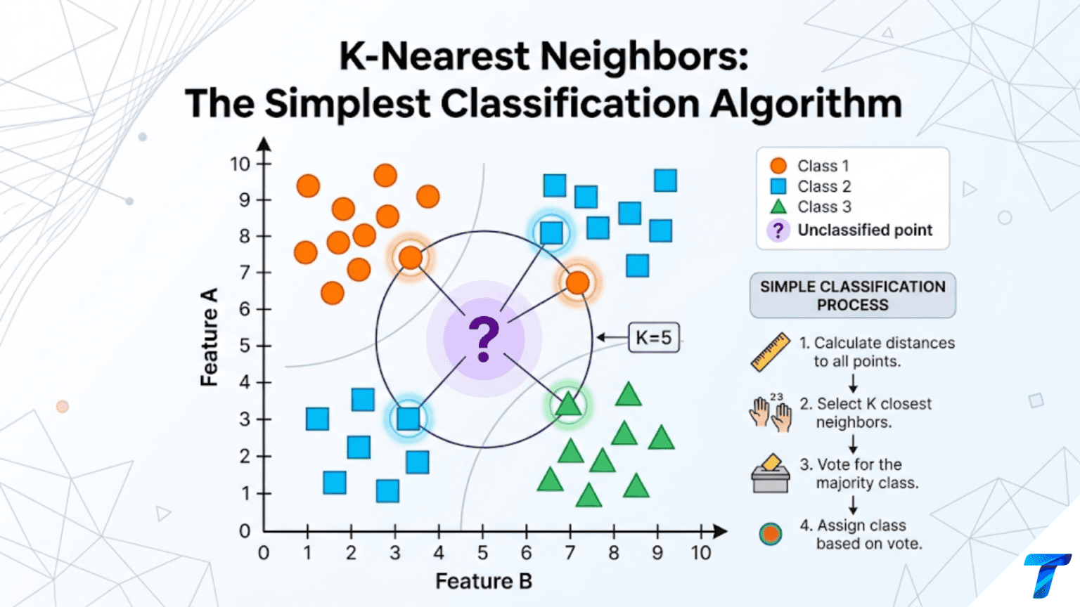
Imagine you move to a new city and want to decide where to live. One perfectly reasonable approach: find the neighborhoods most similar to neighborhoods you already know you like, and move somewhere like those. You are not constructing an elaborate mathematical model of your housing preferences — you are simply reasoning by analogy, asking “what are the closest matches to what I already know?”
This is exactly how K-Nearest Neighbors works. It is one of the most intuitive machine learning algorithms imaginable, and also one of the oldest. When asked to classify a new data point, KNN looks at the K training examples that are most similar to it and predicts the majority class among those neighbors. Nothing is computed during training — the algorithm simply memorizes the dataset and does all its work at prediction time.
Despite its simplicity, KNN is genuinely useful. It requires no assumptions about the shape of the decision boundary, naturally handles multi-class problems, and can approximate arbitrarily complex classification surfaces given enough data. Understanding KNN deeply — why it works, where it fails, and what governs its behavior — builds foundational intuition that carries through to more complex algorithms.
This article develops a complete understanding of KNN: the core algorithm, the mathematics of distance, the critical role of K, how to implement it from scratch, its strengths and limitations, and how to use it effectively with scikit-learn.
The Core Idea: Classification by Analogy
A Concrete Example
Suppose you are building a system to classify whether a customer will churn based on two features: their monthly spending and their number of support tickets. Your training set contains 1,000 labeled customers (churned or retained). A new customer arrives with spending = $85/month and 3 support tickets. Will they churn?
KNN’s answer: find the K customers in your training set whose (spending, tickets) values are most similar to (85, 3), look at how those customers turned out, and predict the majority outcome.
With K=5, you might find that 4 of the 5 nearest customers churned and 1 did not. KNN predicts: churn.
With K=1, you find only the single most similar customer. If they churned, you predict churn. This is extremely sensitive to individual data points.
With K=100, you average over a much larger neighborhood. The prediction is smoother and more stable, but may blur decision boundaries.
The choice of K is the single most important decision in KNN and is the subject of an entire separate article (Article 73). Here we focus on the algorithm itself.
The Algorithm: Step by Step
The KNN prediction process for a new query point x:
Step 1: Compute distances. Calculate the distance from x to every training point.
Step 2: Find K nearest neighbors. Sort training points by distance and take the K smallest.
Step 3: Majority vote. Count the class labels among the K neighbors. The most frequent class is the prediction.
Step 4 (optional): Weighted vote. Weight each neighbor’s vote by 1/distance, so closer neighbors have more influence.
Mathematical Expression
Given a query point x, training set {(x₁, y₁), …, (xₙ, yₙ)}, and a distance function d(·,·):
where N_K(x) is the set of K training indices with the smallest distances to x.
Distance Metrics: The Heart of KNN
The concept of “nearest” is only meaningful once you define what “near” means. The choice of distance metric can dramatically change which neighbors are found — and therefore the predictions.
Euclidean Distance (L2)
The straight-line distance between two points in n-dimensional space:
This is the default and most commonly used metric. It treats all dimensions equally and works well when features have similar scales and the notion of “closeness” corresponds to geometric proximity.
Manhattan Distance (L1)
The sum of absolute differences along each dimension:
Named after navigating a grid of city blocks — you can only move horizontally or vertically. Manhattan distance is less sensitive to large differences in a single dimension and can perform better when features have different units or contain outliers.
Minkowski Distance (Generalization)
Both Euclidean (p=2) and Manhattan (p=1) are special cases of the Minkowski distance:
As p → ∞, this becomes the Chebyshev distance: the maximum absolute difference along any single dimension.
Hamming Distance
For categorical features, Hamming distance counts the number of positions where two vectors differ:
import numpy as np
import matplotlib.pyplot as plt

def euclidean_distance(a, b):
    """Standard Euclidean (L2) distance."""
    return np.sqrt(np.sum((np.array(a) - np.array(b)) ** 2))

def manhattan_distance(a, b):
    """Manhattan (L1) distance."""
    return np.sum(np.abs(np.array(a) - np.array(b)))

def minkowski_distance(a, b, p):
    """Minkowski distance with parameter p."""
    return np.sum(np.abs(np.array(a) - np.array(b)) ** p) ** (1 / p)

def cosine_distance(a, b):
    """Cosine distance = 1 - cosine similarity. Good for high-dimensional text/embeddings."""
    a, b = np.array(a, dtype=float), np.array(b, dtype=float)
    dot_product = np.dot(a, b)
    norm_a = np.linalg.norm(a)
    norm_b = np.linalg.norm(b)
    if norm_a == 0 or norm_b == 0:
        return 1.0
    return 1.0 - dot_product / (norm_a * norm_b)


# Demonstrate different distance metrics on same pair of points
a = np.array([0, 0])
b = np.array([3, 4])

print("=== Distance Metrics Comparison ===\n")
print(f"  Point A: {a}")
print(f"  Point B: {b}\n")
print(f"  {'Metric':<25} | {'Distance':>10} | Notes")
print("  " + "-" * 55)
print(f"  {'Euclidean (L2)':<25} | {euclidean_distance(a, b):>10.4f} | √(9+16) = 5")
print(f"  {'Manhattan (L1)':<25} | {manhattan_distance(a, b):>10.4f} | |3|+|4| = 7")
print(f"  {'Minkowski p=3':<25} | {minkowski_distance(a, b, 3):>10.4f} |")
print(f"  {'Chebyshev (p→∞)':<25} | {max(abs(a-b)):>10.4f} | max(3,4) = 4")
print(f"  {'Cosine Distance':<25} | {cosine_distance(a, b):>10.4f} | angle-based")

# Visualize unit circles for different distance metrics
fig, axes = plt.subplots(1, 3, figsize=(14, 5))

theta = np.linspace(0, 2 * np.pi, 500)

# For each metric, plot all points with distance = 1 from origin
for ax, (p, name, color) in zip(axes, [
    (2, "Euclidean (p=2)\nCircular unit ball", "steelblue"),
    (1, "Manhattan (p=1)\nDiamond unit ball", "coral"),
    (float('inf'), "Chebyshev (p→∞)\nSquare unit ball", "mediumseagreen"),
]):
    points = []
    for angle in theta:
        direction = np.array([np.cos(angle), np.sin(angle)])
        # Find point on unit sphere in this metric
        if p == float('inf'):
            # Chebyshev: |max component| = 1
            scale = 1.0 / max(abs(direction))
        else:
            # Minkowski: ||x||_p = 1
            norm_p = np.sum(np.abs(direction) ** p) ** (1 / p)
            scale = 1.0 / norm_p
        points.append(scale * direction)

    points = np.array(points)
    ax.fill(points[:, 0], points[:, 1], alpha=0.3, color=color)
    ax.plot(points[:, 0], points[:, 1], color=color, lw=2.5)
    ax.axhline(0, color='gray', lw=0.8, alpha=0.5)
    ax.axvline(0, color='gray', lw=0.8, alpha=0.5)
    ax.set_aspect('equal')
    ax.set_title(name, fontsize=11, fontweight='bold')
    ax.set_xlim([-1.5, 1.5])
    ax.set_ylim([-1.5, 1.5])
    ax.grid(True, alpha=0.3)

plt.suptitle("Unit Balls for Different Distance Metrics\n"
             "(Points equidistant from origin under each metric)",
             fontsize=13, fontweight='bold')
plt.tight_layout()
plt.savefig("distance_metrics_unit_balls.png", dpi=150, bbox_inches='tight')
plt.show()
print("\nSaved: distance_metrics_unit_balls.png")The Scale Sensitivity Problem
A critical and frequently missed issue: KNN is extremely sensitive to the scale of features. If one feature has values in the range [0, 1] and another has values in [0, 10,000], the second feature will dominate all distance calculations, effectively making the first feature invisible to the algorithm.
import numpy as np

# Demonstrate scale sensitivity
np.random.seed(42)

# Query point and two candidates
query      = np.array([50.0, 0.5])   # [age, height_in_meters]
candidate1 = np.array([51.0, 0.5])   # Age +1, same height  (logically similar)
candidate2 = np.array([50.0, 1.5])   # Same age, height +1m (very different person)

print("=== Scale Sensitivity in KNN ===\n")
print("  Raw features (NOT normalized):")
print(f"  Query:      age={query[0]}, height={query[1]}m")
print(f"  Candidate1: age={candidate1[0]}, height={candidate1[1]}m  (1 year older, same height)")
print(f"  Candidate2: age={candidate2[0]}, height={candidate2[1]}m  (same age, 1 meter taller!)")

d1_raw = euclidean_distance(query, candidate1)
d2_raw = euclidean_distance(query, candidate2)
print(f"\n  Euclidean distances (raw):")
print(f"  Query → Candidate1: {d1_raw:.4f}")
print(f"  Query → Candidate2: {d2_raw:.4f}")
print(f"  KNN picks: Candidate{'1' if d1_raw < d2_raw else '2'} as nearest")
print(f"  (This is {'correct' if d1_raw < d2_raw else 'WRONG — a 1m height diff > 1 year age'})")

# After scaling age to [0,1] and height to [0,1]
age_min, age_max       = 0, 100
height_min, height_max = 0, 2.5

def normalize(val, vmin, vmax):
    return (val - vmin) / (vmax - vmin)

query_n      = np.array([normalize(50,  age_min, age_max), normalize(0.5, height_min, height_max)])
candidate1_n = np.array([normalize(51,  age_min, age_max), normalize(0.5, height_min, height_max)])
candidate2_n = np.array([normalize(50,  age_min, age_max), normalize(1.5, height_min, height_max)])

d1_norm = euclidean_distance(query_n, candidate1_n)
d2_norm = euclidean_distance(query_n, candidate2_n)

print(f"\n  After min-max normalization to [0,1]:")
print(f"  Query → Candidate1: {d1_norm:.4f}")
print(f"  Query → Candidate2: {d2_norm:.4f}")
print(f"  KNN picks: Candidate{'1' if d1_norm < d2_norm else '2'} as nearest")
print(f"\n → ALWAYS normalize features before using KNN!")The rule: Always normalize or standardize features before applying KNN. Min-max scaling or z-score standardization both work; the choice depends on your data distribution and whether outliers are a concern.
KNN from Scratch
Building KNN from scratch in Python reinforces every aspect of the algorithm and makes the moving parts completely transparent.
import numpy as np
from collections import Counter

class KNNClassifier:
    """
    K-Nearest Neighbors Classifier implemented from scratch.

    Supports:
    - Multiple distance metrics (euclidean, manhattan, minkowski)
    - Uniform and distance-weighted voting
    - Multi-class classification
    """

    def __init__(self, k=5, metric='euclidean', weights='uniform', p=2):
        """
        Args:
            k:       Number of neighbors to consider
            metric:  Distance metric: 'euclidean', 'manhattan', 'minkowski', 'cosine'
            weights: 'uniform' (equal votes) or 'distance' (closer = more vote)
            p:       Minkowski parameter (only used when metric='minkowski')
        """
        self.k       = k
        self.metric  = metric
        self.weights = weights
        self.p       = p
        self.X_train = None
        self.y_train = None

    def fit(self, X, y):
        """
        Store training data. KNN has no actual training step.

        Args:
            X: Feature matrix of shape (n_samples, n_features)
            y: Target labels of shape (n_samples,)
        """
        self.X_train = np.array(X, dtype=float)
        self.y_train = np.array(y)
        self.classes_ = np.unique(y)
        return self

    def _compute_distances(self, x):
        """Compute distances from query point x to all training points."""
        if self.metric == 'euclidean':
            # Vectorized: avoids Python loop over training points
            diff = self.X_train - x
            return np.sqrt(np.sum(diff ** 2, axis=1))

        elif self.metric == 'manhattan':
            diff = self.X_train - x
            return np.sum(np.abs(diff), axis=1)

        elif self.metric == 'minkowski':
            diff = self.X_train - x
            return np.sum(np.abs(diff) ** self.p, axis=1) ** (1 / self.p)

        elif self.metric == 'cosine':
            # Cosine distance = 1 - cosine similarity
            norms_train = np.linalg.norm(self.X_train, axis=1)
            norm_x      = np.linalg.norm(x)
            # Guard against zero vectors
            denom = norms_train * norm_x
            denom[denom == 0] = 1e-10
            similarities = self.X_train @ x / denom
            return 1.0 - similarities

        else:
            raise ValueError(f"Unknown metric: {self.metric}")

    def _predict_single(self, x):
        """Predict class for a single query point."""
        distances = self._compute_distances(x)

        # Get indices of K nearest neighbors
        k_nearest_idx = np.argsort(distances)[:self.k]
        k_nearest_labels = self.y_train[k_nearest_idx]
        k_nearest_dists  = distances[k_nearest_idx]

        if self.weights == 'uniform':
            # Simple majority vote
            vote_counts = Counter(k_nearest_labels)
            return vote_counts.most_common(1)[0][0]

        elif self.weights == 'distance':
            # Weight each vote by 1/distance (closer neighbors count more)
            # Handle zero distance (exact match)
            k_nearest_dists = np.where(k_nearest_dists == 0,
                                        1e-10, k_nearest_dists)
            vote_weights = 1.0 / k_nearest_dists

            # Accumulate weighted votes per class
            class_weights = {}
            for label, weight in zip(k_nearest_labels, vote_weights):
                class_weights[label] = class_weights.get(label, 0) + weight

            return max(class_weights, key=class_weights.get)

        else:
            raise ValueError(f"Unknown weights: {self.weights}")

    def predict(self, X):
        """
        Predict class labels for multiple samples.

        Args:
            X: Feature matrix of shape (n_queries, n_features)

        Returns:
            Predicted labels array of shape (n_queries,)
        """
        X = np.array(X, dtype=float)
        return np.array([self._predict_single(x) for x in X])

    def predict_proba(self, X):
        """
        Predict class probabilities (fraction of K neighbors in each class).

        Args:
            X: Feature matrix of shape (n_queries, n_features)

        Returns:
            Probability matrix of shape (n_queries, n_classes)
        """
        X = np.array(X, dtype=float)
        probas = []

        for x in X:
            distances = self._compute_distances(x)
            k_nearest_idx    = np.argsort(distances)[:self.k]
            k_nearest_labels = self.y_train[k_nearest_idx]
            k_nearest_dists  = distances[k_nearest_idx]

            class_votes = {}

            if self.weights == 'uniform':
                for label in k_nearest_labels:
                    class_votes[label] = class_votes.get(label, 0) + 1
                total = self.k
            else:
                k_nearest_dists = np.where(k_nearest_dists == 0,
                                            1e-10, k_nearest_dists)
                vote_weights = 1.0 / k_nearest_dists
                for label, weight in zip(k_nearest_labels, vote_weights):
                    class_votes[label] = class_votes.get(label, 0) + weight
                total = sum(vote_weights)

            row = [class_votes.get(c, 0) / total for c in self.classes_]
            probas.append(row)

        return np.array(probas)

    def score(self, X, y):
        """Accuracy score."""
        return np.mean(self.predict(X) == np.array(y))


# Test the implementation
from sklearn.datasets import make_classification, make_blobs
from sklearn.model_selection import train_test_split
from sklearn.preprocessing import StandardScaler
from sklearn.neighbors import KNeighborsClassifier as SklearnKNN

np.random.seed(42)
X_test_data, y_test_data = make_classification(
    n_samples=500, n_features=4, n_informative=3,
    n_classes=3, n_clusters_per_class=1, random_state=42
)

X_tr, X_te, y_tr, y_te = train_test_split(
    X_test_data, y_test_data, test_size=0.25, random_state=42, stratify=y_test_data
)

scaler = StandardScaler()
X_tr_s = scaler.fit_transform(X_tr)
X_te_s = scaler.transform(X_te)

print("=== KNN from Scratch vs Scikit-learn ===\n")
for k in [3, 5, 10]:
    # Our implementation
    our_knn = KNNClassifier(k=k, metric='euclidean', weights='uniform')
    our_knn.fit(X_tr_s, y_tr)
    our_acc = our_knn.score(X_te_s, y_te)

    # Scikit-learn reference
    sk_knn = SklearnKNN(n_neighbors=k, metric='euclidean', weights='uniform')
    sk_knn.fit(X_tr_s, y_tr)
    sk_acc = sk_knn.score(X_te_s, y_te)

    match = "✓ Match" if abs(our_acc - sk_acc) < 0.001 else "✗ Mismatch"
print(f" K={k:2d}: Our={our_acc:.4f} Sklearn={sk_acc:.4f} {match}")Visualizing KNN Decision Boundaries
One of the best ways to build intuition for KNN is to visualize how the decision boundary changes as K varies.
import numpy as np
import matplotlib.pyplot as plt
from sklearn.datasets import make_classification, make_moons, make_circles
from sklearn.preprocessing import StandardScaler

def plot_knn_decision_boundary(X, y, k_values, dataset_name, figsize=(16, 5)):
    """
    Plot KNN decision boundaries for multiple K values side by side.
    Shows how increasing K smooths the boundary.
    """
    scaler_vis = StandardScaler()
    X_scaled = scaler_vis.fit_transform(X)

    colors = ['steelblue', 'coral', 'mediumseagreen', 'mediumpurple']

    fig, axes = plt.subplots(1, len(k_values), figsize=figsize)
    if len(k_values) == 1:
        axes = [axes]

    x_min, x_max = X_scaled[:, 0].min() - 0.5, X_scaled[:, 0].max() + 0.5
    y_min, y_max = X_scaled[:, 1].min() - 0.5, X_scaled[:, 1].max() + 0.5

    xx, yy = np.meshgrid(
        np.linspace(x_min, x_max, 200),
        np.linspace(y_min, y_max, 200)
    )
    grid_points = np.c_[xx.ravel(), yy.ravel()]

    for ax, k in zip(axes, k_values):
        knn_vis = KNNClassifier(k=k)
        knn_vis.fit(X_scaled, y)

        Z = knn_vis.predict(grid_points).reshape(xx.shape)

        ax.contourf(xx, yy, Z, alpha=0.25,
                    colors=[colors[c] for c in range(len(np.unique(y)))])
        ax.contour(xx, yy, Z, colors='black', linewidths=0.8, alpha=0.4)

        for cls, color in zip(np.unique(y), colors):
            mask = y == cls
            ax.scatter(X_scaled[mask, 0], X_scaled[mask, 1],
                      c=color, edgecolors='white', s=40, linewidth=0.5,
                      label=f'Class {cls}', alpha=0.85)

        ax.set_title(f'K = {k}', fontsize=13, fontweight='bold')
        ax.set_xlabel('Feature 1', fontsize=10)
        ax.set_ylabel('Feature 2', fontsize=10)
        ax.legend(fontsize=8, loc='upper right')
        ax.grid(True, alpha=0.2)

    plt.suptitle(f'KNN Decision Boundaries: {dataset_name}\n'
                 '(Small K = complex boundary, large K = smooth boundary)',
                 fontsize=13, fontweight='bold', y=1.02)
    plt.tight_layout()
    plt.savefig(f"knn_boundary_{dataset_name.replace(' ', '_')}.png",
                dpi=150, bbox_inches='tight')
    plt.show()
    print(f"Saved: knn_boundary_{dataset_name.replace(' ', '_')}.png")


# Visualize on three datasets
np.random.seed(42)

# Dataset 1: Two moons (nonlinear boundary)
X_moons, y_moons = make_moons(n_samples=300, noise=0.25, random_state=42)
plot_knn_decision_boundary(X_moons, y_moons, k_values=[1, 5, 20, 50],
                            dataset_name="Two Moons")

# Dataset 2: Concentric circles (highly nonlinear)
X_circles, y_circles = make_circles(n_samples=300, noise=0.15, factor=0.5, random_state=42)
plot_knn_decision_boundary(X_circles, y_circles, k_values=[1, 5, 15, 50],
dataset_name="Concentric Circles")The visualization reveals the fundamental tradeoff: K=1 produces a jagged boundary that perfectly separates training data but overfits to noise. Large K produces smooth, stable boundaries that may underfit complex true boundaries. The optimal K sits somewhere between these extremes.
Strengths and Limitations
Strengths
No training phase. KNN is a lazy learner — it stores training data and does all computation at prediction time. This means model updates (adding new data) are trivially easy: just add the new points to the stored dataset without retraining anything.
Non-parametric flexibility. KNN makes no assumptions about the functional form of the decision boundary. It can learn any shape: linear, circular, sinusoidal, arbitrary clusters. Complex non-linear boundaries that defeat logistic regression are often handled naturally by KNN.
Naturally multi-class. Unlike some algorithms that require one-vs-rest wrappers for multi-class problems, KNN handles any number of classes with no modification.
Interpretable predictions. When KNN makes a prediction, you can directly inspect the K neighbors that drove it. This is genuine local interpretability — you can point to specific training examples and say “these are the cases most like yours.”
Effective on small datasets. With small training sets (hundreds to low thousands of samples), KNN often competes with or outperforms more sophisticated algorithms that need more data to estimate their parameters reliably.
Limitations
Prediction is slow. Computing distances to every training point for each new query takes O(n × d) time, where n is training size and d is dimensionality. For a training set of 1 million points with 100 features, each prediction requires 100 million multiplications. This is prohibitive in real-time applications.
High memory usage. The entire training dataset must be stored in memory. For large datasets, this is costly.
Curse of dimensionality. As the number of features grows, the concept of “nearest” breaks down. In high dimensions, all points become approximately equidistant from any query point — there are no true nearest neighbors, just points that happen to be slightly less far away than others. KNN degrades sharply beyond roughly 10–20 informative features.
Sensitive to irrelevant features. Every feature contributes equally to distance calculations. If 90 of your 100 features are irrelevant noise, the distances computed are mostly measuring noise rather than meaningful similarity.
Sensitive to feature scale. As demonstrated above, features with large numerical ranges dominate the distance calculation. Normalization is mandatory.
Poor performance on imbalanced data. If 95% of training points are class 0, the K nearest neighbors to almost any query will include mostly class 0 points — not because those are the true nearest matches, but simply because they are everywhere.
KNN with Scikit-learn
For production use, scikit-learn’s KNeighborsClassifier is highly optimized with efficient data structures (KD-trees and ball trees) that reduce prediction time from O(n) to O(log n) for lower-dimensional data.
from sklearn.neighbors import KNeighborsClassifier
from sklearn.datasets import load_wine
from sklearn.model_selection import train_test_split, cross_val_score
from sklearn.preprocessing import StandardScaler
from sklearn.pipeline import Pipeline
from sklearn.metrics import classification_report, confusion_matrix
import numpy as np
import matplotlib.pyplot as plt
import seaborn as sns

# Wine dataset: 3 classes, 13 chemical features
wine = load_wine()
X_wine, y_wine = wine.data, wine.target

print("=== KNN on Wine Dataset ===\n")
print(f"  Samples: {X_wine.shape[0]}, Features: {X_wine.shape[1]}, Classes: {len(np.unique(y_wine))}")
print(f"  Class distribution: {np.bincount(y_wine)}\n")

X_tr_w, X_te_w, y_tr_w, y_te_w = train_test_split(
    X_wine, y_wine, test_size=0.25, random_state=42, stratify=y_wine
)

# KNN pipeline with normalization
knn_pipeline = Pipeline([
    ('scaler', StandardScaler()),
    ('knn', KNeighborsClassifier(
        n_neighbors=7,
        metric='euclidean',
        weights='distance',    # Closer neighbors get more vote
        algorithm='auto',      # sklearn picks KD-tree or ball tree automatically
        n_jobs=-1
    ))
])

knn_pipeline.fit(X_tr_w, y_tr_w)
y_pred_w = knn_pipeline.predict(X_te_w)

print("=== Classification Report ===\n")
print(classification_report(y_te_w, y_pred_w, target_names=wine.target_names))

# Cross-validation for robust estimate
cv_scores = cross_val_score(knn_pipeline, X_wine, y_wine, cv=10, scoring='accuracy')
print(f"  10-Fold CV Accuracy: {cv_scores.mean():.4f} ± {cv_scores.std():.4f}")

# Confusion matrix
cm = confusion_matrix(y_te_w, y_pred_w)
plt.figure(figsize=(7, 5))
sns.heatmap(cm, annot=True, fmt='d', cmap='Blues',
            xticklabels=wine.target_names,
            yticklabels=wine.target_names,
            linewidths=2, linecolor='white')
plt.title('KNN Confusion Matrix: Wine Classification\n(K=7, distance-weighted)',
          fontsize=12, fontweight='bold')
plt.ylabel('Actual', fontsize=11)
plt.xlabel('Predicted', fontsize=11)
plt.tight_layout()
plt.savefig("knn_wine_confusion_matrix.png", dpi=150)
plt.show()
print("Saved: knn_wine_confusion_matrix.png")
Algorithm Parameter: KD-Tree vs Ball Tree
Scikit-learn’s algorithm parameter selects the data structure used to accelerate neighbor search:
| Algorithm | Time Complexity | Best For |
|---|---|---|
brute | O(n×d) per query | Small datasets, high dimensions |
kd_tree | O(log n) per query | Low dimensions (d ≤ 20), moderate n |
ball_tree | O(log n) per query | Higher dimensions, sparse data |
auto | sklearn decides | Use this in practice |
For datasets with more than ~20 features, KD-tree performance degrades and scikit-learn automatically switches to brute force. The ball_tree algorithm handles slightly higher dimensions but also degrades past ~30–50 features.
The Curse of Dimensionality in Depth
The phrase “curse of dimensionality” was coined by Richard Bellman in 1961 to describe the exponential growth of the volume of space as dimensionality increases. For KNN specifically, it has a concrete and devastating implication: in high dimensions, every point is far from every other point, and the K nearest neighbors of a query point may not be meaningfully “near” at all.
Why Distance Loses Meaning in High Dimensions
In 1 dimension, if you want to capture 10% of the data range, you need to look at a segment covering 10% of the axis. In 2D, to capture 10% of the area, you need a square with side length 10%^(1/2) ≈ 32%. In 10D, to capture 10% of the volume, you need a hypercube with side length 10%^(1/10) ≈ 79%. In 100D, you need side length 10%^(1/100) ≈ 97.7%.
In other words, to find the 10% nearest neighbors in 100 dimensions, you have to look at nearly the entire feature space. Neighbors are no longer local — they are essentially random samples from the full training distribution.
import numpy as np
import matplotlib.pyplot as plt

def demonstrate_curse_of_dimensionality(n_samples=1000, n_trials=50):
    """
    Demonstrate how nearest neighbor distances concentrate in high dimensions.

    Shows that the ratio of (farthest neighbor / nearest neighbor) approaches 1
    as dimensions increase, meaning all points become equidistant.
    """
    dimensions = [1, 2, 3, 5, 10, 20, 50, 100, 200, 500]

    dist_ratios  = []   # max_dist / min_dist for K=10 neighbors
    relative_gaps = []  # (max - min) / mean  — normalized spread

    for d in dimensions:
        trial_ratios = []

        for _ in range(n_trials):
            # Random points uniformly in d-dimensional unit hypercube
            X_d = np.random.uniform(0, 1, size=(n_samples, d))

            # Pick a random query point
            query = np.random.uniform(0, 1, size=d)

            # Compute distances to all training points
            dists = np.sqrt(np.sum((X_d - query) ** 2, axis=1))
            dists_sorted = np.sort(dists)

            # Ratio of 10th nearest to 1st nearest
            d_min = dists_sorted[1]    # Skip index 0 (could be self)
            d_max = dists_sorted[10]

            if d_min > 0:
                trial_ratios.append(d_max / d_min)

        dist_ratios.append(np.mean(trial_ratios))

    # Also compute: concentration of distances (std/mean)
    concentration = []
    for d in dimensions:
        sample_dists = []
        for _ in range(20):
            X_d = np.random.uniform(0, 1, size=(500, d))
            query = np.random.uniform(0, 1, size=d)
            dists = np.sqrt(np.sum((X_d - query) ** 2, axis=1))
            # Relative spread: std / mean
            if dists.mean() > 0:
                sample_dists.append(dists.std() / dists.mean())
        concentration.append(np.mean(sample_dists))

    fig, axes = plt.subplots(1, 2, figsize=(14, 5))

    axes[0].semilogx(dimensions, dist_ratios, 'o-', color='coral',
                     linewidth=2.5, markersize=8)
    axes[0].axhline(y=1.0, color='gray', linestyle='--', lw=1.5,
                    label='Ratio=1: all points equidistant')
    axes[0].set_xlabel("Number of Dimensions (log scale)", fontsize=12)
    axes[0].set_ylabel("Ratio: 10th Nearest / 1st Nearest Distance", fontsize=12)
    axes[0].set_title("Distance Concentration:\n"
                       "As dimensions grow, all neighbors become equally far",
                       fontsize=12, fontweight='bold')
    axes[0].legend(fontsize=9)
    axes[0].grid(True, alpha=0.3)

    axes[1].semilogx(dimensions, concentration, 's-', color='steelblue',
                     linewidth=2.5, markersize=8)
    axes[1].set_xlabel("Number of Dimensions (log scale)", fontsize=12)
    axes[1].set_ylabel("Relative Spread (Std/Mean of distances)", fontsize=12)
    axes[1].set_title("Distance Spread Collapses in High Dimensions:\n"
                       "All points become nearly the same distance apart",
                       fontsize=12, fontweight='bold')
    axes[1].grid(True, alpha=0.3)

    plt.suptitle("The Curse of Dimensionality: KNN Degrades in High Dimensions",
                 fontsize=13, fontweight='bold', y=1.01)
    plt.tight_layout()
    plt.savefig("curse_of_dimensionality.png", dpi=150, bbox_inches='tight')
    plt.show()
    print("Saved: curse_of_dimensionality.png")

    print(f"\n  {'Dimensions':>12} | {'Ratio (10th/1st)':>17} | {'Relative Spread':>16}")
    print("  " + "-" * 50)
    for d, ratio, conc in zip(dimensions, dist_ratios, concentration):
        print(f"  {d:>12} | {ratio:>17.3f} | {conc:>16.4f}")

    print("\n  As dimensions grow:")
    print("  - Ratio → 1: nearest and farthest neighbors at same distance")
    print("  - Spread → 0: all distances become identical")
    print("  - Result: 'nearest' neighbors are no more similar than random points")

np.random.seed(42)
demonstrate_curse_of_dimensionality()Practical Dimensionality Thresholds
In practice, KNN degrades noticeably above roughly 10–20 features. The standard mitigations are:
Dimensionality reduction before KNN. Apply PCA to reduce to the most informative principal components before computing distances. This removes noise dimensions that pollute the distance metric while preserving structure.
Feature selection. Remove features with low predictive power before applying KNN. A random forest’s feature importance scores provide a fast ranking.
Feature weighting. Instead of treating all features equally, weight each feature’s contribution to the distance by its estimated relevance (e.g., its correlation with the target). This is effectively learned metric learning.
from sklearn.decomposition import PCA
from sklearn.pipeline import Pipeline
from sklearn.preprocessing import StandardScaler
from sklearn.neighbors import KNeighborsClassifier
from sklearn.datasets import make_classification
from sklearn.model_selection import cross_val_score
import numpy as np

np.random.seed(42)

# High-dimensional dataset: 100 features, only 5 are informative
X_hd, y_hd = make_classification(
    n_samples=1000, n_features=100, n_informative=5,
    n_redundant=5, n_repeated=0, random_state=42
)

print("=== KNN with Dimensionality Reduction ===\n")
print(f"  Dataset: {X_hd.shape[1]} features, only 5 are informative\n")
print(f"  {'Strategy':<40} | {'5-Fold AUC':>12} | {'Std':>7}")
print("  " + "-" * 65)

strategies = [
    ("KNN (no scaling, all 100 features)",
     Pipeline([('knn', KNeighborsClassifier(n_neighbors=7))])),
    ("KNN (scaled, all 100 features)",
     Pipeline([('sc', StandardScaler()),
               ('knn', KNeighborsClassifier(n_neighbors=7))])),
    ("KNN (scaled + PCA 20 components)",
     Pipeline([('sc', StandardScaler()),
               ('pca', PCA(n_components=20)),
               ('knn', KNeighborsClassifier(n_neighbors=7))])),
    ("KNN (scaled + PCA 5 components)",
     Pipeline([('sc', StandardScaler()),
               ('pca', PCA(n_components=5)),
               ('knn', KNeighborsClassifier(n_neighbors=7))])),
]

for name, pipe in strategies:
    scores = cross_val_score(pipe, X_hd, y_hd, cv=5, scoring='roc_auc', n_jobs=-1)
    print(f"  {name:<40} | {scores.mean():>12.4f} | {scores.std():>7.4f}")

print("\n PCA before KNN substantially improves performance on high-dimensional data.")Weighted KNN: Giving Closer Neighbors More Influence
Standard KNN gives each of the K neighbors an equal vote regardless of how close they are. A neighbor at distance 0.01 and one at distance 10 both count equally. This can hurt predictions when there is a wide spread in distances among the K neighbors.
Distance-weighted KNN assigns each neighbor a vote weight of 1/distance (or 1/distance²). The prediction is still the class with the highest total weight, but now proximity matters:
import numpy as np
import matplotlib.pyplot as plt
from sklearn.neighbors import KNeighborsClassifier
from sklearn.datasets import make_moons, make_classification
from sklearn.preprocessing import StandardScaler
from sklearn.model_selection import cross_val_score
from sklearn.pipeline import Pipeline

np.random.seed(42)
X_wt, y_wt = make_moons(n_samples=400, noise=0.30, random_state=42)

print("=== Uniform vs Distance-Weighted KNN ===\n")
print(f"  {'K':>4} | {'Uniform CV Acc':>16} | {'Distance-Weighted CV Acc':>25} | {'Improvement'}")
print("  " + "-" * 72)

for k in [1, 3, 5, 7, 10, 15, 25]:
    pipe_uniform = Pipeline([
        ('sc', StandardScaler()),
        ('knn', KNeighborsClassifier(n_neighbors=k, weights='uniform'))
    ])
    pipe_dist = Pipeline([
        ('sc', StandardScaler()),
        ('knn', KNeighborsClassifier(n_neighbors=k, weights='distance'))
    ])

    acc_u = cross_val_score(pipe_uniform, X_wt, y_wt, cv=5, scoring='accuracy')
    acc_d = cross_val_score(pipe_dist,    X_wt, y_wt, cv=5, scoring='accuracy')

    improvement = acc_d.mean() - acc_u.mean()
    flag = "↑" if improvement > 0.002 else "~"
    print(f"  {k:>4} | {acc_u.mean():>16.4f} | {acc_d.mean():>25.4f} | {improvement:+.4f} {flag}")

print("\n  Distance weighting most helps when K is large (more diversity among neighbors).")

# Visualize uniform vs weighted boundary at same K
fig, axes = plt.subplots(1, 2, figsize=(14, 5))

scaler_wt = StandardScaler()
X_wt_s = scaler_wt.fit_transform(X_wt)

x_min, x_max = X_wt_s[:, 0].min() - 0.5, X_wt_s[:, 0].max() + 0.5
y_min_v, y_max_v = X_wt_s[:, 1].min() - 0.5, X_wt_s[:, 1].max() + 0.5
xx_v, yy_v = np.meshgrid(np.linspace(x_min, x_max, 300),
                          np.linspace(y_min_v, y_max_v, 300))
grid_v = np.c_[xx_v.ravel(), yy_v.ravel()]

for ax, weight_type, title in [
    (axes[0], 'uniform',  'Uniform Weights (K=15)\nEach of 15 neighbors votes equally'),
    (axes[1], 'distance', 'Distance Weights (K=15)\nCloser neighbors vote more'),
]:
    knn_v = KNeighborsClassifier(n_neighbors=15, weights=weight_type)
    knn_v.fit(X_wt_s, y_wt)
    Z_v = knn_v.predict(grid_v).reshape(xx_v.shape)

    ax.contourf(xx_v, yy_v, Z_v, alpha=0.25, colors=['steelblue', 'coral'])
    ax.contour(xx_v, yy_v, Z_v, colors='black', linewidths=1.0, alpha=0.5)

    for cls, color in [(0, 'steelblue'), (1, 'coral')]:
        mask = y_wt == cls
        ax.scatter(X_wt_s[mask, 0], X_wt_s[mask, 1],
                  c=color, edgecolors='white', s=40, linewidth=0.5, alpha=0.85)

    ax.set_title(title, fontsize=11, fontweight='bold')
    ax.set_xlabel("Feature 1", fontsize=10)
    ax.set_ylabel("Feature 2", fontsize=10)
    ax.grid(True, alpha=0.2)

plt.suptitle("Uniform vs Distance-Weighted KNN: Two Moons Dataset",
             fontsize=13, fontweight='bold')
plt.tight_layout()
plt.savefig("knn_uniform_vs_distance_weighted.png", dpi=150)
plt.show()
print("Saved: knn_uniform_vs_distance_weighted.png")Distance-weighted KNN tends to outperform uniform KNN when K is larger, because larger K neighborhoods contain more distant points — giving uniform voting, where distant points count equally, increasingly poor signal. With distance weighting, the prediction is still dominated by the truly close neighbors, while distant ones merely add a small tiebreaking signal.
KNN for Regression
KNN extends naturally to regression: instead of majority voting, predict the mean (or weighted mean) of the K nearest neighbors’ target values.
from sklearn.neighbors import KNeighborsRegressor
from sklearn.datasets import fetch_california_housing
from sklearn.model_selection import train_test_split, cross_val_score
from sklearn.preprocessing import StandardScaler
from sklearn.pipeline import Pipeline
from sklearn.metrics import mean_squared_error, r2_score
import numpy as np

housing = fetch_california_housing()
X_h, y_h = housing.data, housing.target

X_tr_h, X_te_h, y_tr_h, y_te_h = train_test_split(
    X_h, y_h, test_size=0.20, random_state=42
)

knn_reg = Pipeline([
    ('scaler', StandardScaler()),
    ('knn', KNeighborsRegressor(
        n_neighbors=10,
        weights='distance',
        algorithm='auto',
        n_jobs=-1
    ))
])

knn_reg.fit(X_tr_h, y_tr_h)
y_pred_h = knn_reg.predict(X_te_h)

rmse = np.sqrt(mean_squared_error(y_te_h, y_pred_h))
r2   = r2_score(y_te_h, y_pred_h)

print("=== KNN Regression: California Housing ===\n")
print(f"  K=10, distance-weighted")
print(f"  RMSE: {rmse:.4f}")
print(f"  R²:   {r2:.4f}")

# Show how K affects regression performance
print(f"\n  K sweep (5-Fold CV):")
print(f"  {'K':>5} | {'Mean R²':>9} | {'Std':>7}")
print("  " + "-" * 28)

for k in [1, 3, 5, 10, 20, 50]:
    pipe_k = Pipeline([
        ('scaler', StandardScaler()),
        ('knn', KNeighborsRegressor(n_neighbors=k, weights='distance', n_jobs=-1))
    ])
    scores = cross_val_score(pipe_k, X_h, y_h, cv=5, scoring='r2')
print(f" {k:>5} | {scores.mean():>9.4f} | {scores.std():>7.4f}")Practical Guidelines
Always scale features first. Make this an automatic habit. Wrap KNN in a Pipeline with StandardScaler or MinMaxScaler. Unscaled KNN is broken by definition.
Use weighted voting for cleaner boundaries. Setting weights='distance' in scikit-learn makes predictions smoother and reduces the sensitivity of the boundary to the exact value of K.
Choose K with cross-validation. Never set K to 5 because it is a default. Run a cross-validated sweep over K values and pick the one that maximizes validation performance. Article 73 covers this in depth.
Feature selection matters more than for most algorithms. Irrelevant features actively harm KNN by polluting distance calculations with noise. A brief feature selection step (correlation analysis, mutual information, or a quick random forest importance ranking) before KNN can produce substantial improvements.
Consider approximate nearest neighbors for large datasets. Libraries like Faiss, Annoy, and HNSW implement approximate nearest neighbor search that runs in sub-linear time with small accuracy tradeoffs — making KNN practical at scales where exact search is infeasible.
KNN shines in local pattern problems. When the relationship between features and labels is highly local (the right class depends on very specific feature combinations that vary across the feature space), KNN often outperforms global models like logistic regression.
Summary
K-Nearest Neighbors is remarkable for combining extreme conceptual simplicity with genuine practical utility. The algorithm has essentially two moving parts: a distance metric that defines similarity and a value of K that controls how much of the local neighborhood to consider.
This simplicity is both its strength and its limitation. Because KNN makes no assumptions about the global structure of the data, it adapts naturally to any decision boundary shape. Because it relies entirely on local distance relationships, it fails when those relationships are masked by irrelevant features, obscured by scale mismatches, or stretched impossibly thin in high-dimensional space.
The key practical habits — always normalize, always tune K via cross-validation, always select features — transform KNN from a naive algorithm that sometimes fails to a reliable baseline that often performs surprisingly well. Many practitioners keep KNN as a permanent first-pass baseline when evaluating new datasets: it is fast to implement, interpretable by inspection, and often competitive enough to benchmark against.
Understanding KNN also builds foundations for more advanced algorithms. Kernel methods, radial basis function networks, and locally-weighted regression all share the same fundamental insight that predictions should be guided by the most similar training examples. The curse of dimensionality that plagues KNN motivates dimensionality reduction and representation learning. The slowness of exact neighbor search motivates the approximate search data structures that power modern recommendation systems and vector databases.