Current draw is the rate at which a robot’s electrical components consume charge from the battery, measured in milliamps (mA) or amps (A), and it directly determines how long a robot runs before the battery is depleted—a robot consuming 2A average from a 2000mAh battery will run for approximately one hour under ideal conditions, but real-world runtime is often far shorter because motors draw many times their average current during startup and stall, components run continuously when they could sleep, and inefficient power conversion wastes energy as heat before it ever reaches the loads it was meant to power.
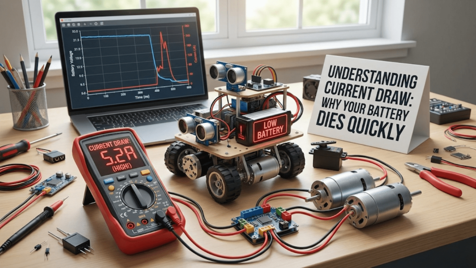
You charged the battery fully. You ran the robot for what felt like no time at all. Now the low-voltage alarm is going off and the robot is slowing down. The rated capacity was 3000mAh — surely that should last longer than fifteen minutes?
This experience is nearly universal in robotics, and it almost always reveals the same lesson: the gap between theoretical battery runtime and actual runtime is caused by current draw that is much higher than expected. Understanding where that current goes — and why it goes there in much larger quantities than advertised specifications suggest — transforms battery life from a mystery into a predictable, manageable engineering parameter.
Current draw is the single most important number for predicting robot runtime. Every component that draws current is a drain on the battery. The sum of all those drains, integrated over time, equals the capacity consumed. When the consumed capacity equals the battery’s rated capacity, the run is over. This seems simple, but the details of how each component draws current — especially motors, which dominate most robots’ power budgets — contain surprises that catch nearly every builder off guard the first time.
This article gives you the complete picture: where current actually goes in a robot, why the real numbers are so much larger than the datasheet minimums, how to measure actual current draw, and practical techniques for stretching battery life without sacrificing performance.
The Current Draw Hierarchy: Who Is Consuming Your Battery
In most mobile robots, current consumers fall into a clear hierarchy based on how much they draw and how much that draw varies during operation.
Tier 1: Drive Motors (Dominant Consumer)
Drive motors are almost always the largest current consumers in a mobile robot, often accounting for 60–80% of total current draw during active operation. This dominance comes from two factors: motors must convert electrical energy into mechanical work against real-world loads, and DC motors are inherently inefficient at typical operating points, with significant current consumed even at no load.
What makes motor current difficult to estimate is its extreme variability. A motor’s current draw depends on the torque it’s producing, which depends on the load it’s driving, which changes every second as the robot accelerates, turns, climbs inclines, or encounters friction:
Motor current vs. operating condition (example: Pololu 150:1 gearmotor):
Stall (blocked rotor):       ~1800 mA  ← wire sizing limit
Climbing steep ramp (70%):    ~900 mA
Normal driving (30% load):    ~350 mA
No-load (free spinning):      ~120 mA
Stationary, motor powered:    ~120 mA  (holding current through driver)
Stationary, driver disabled:   ~0 mA

For two motors on a typical robot:
Worst case (both stalling):   ~3600 mA peak
Typical driving:              ~700 mA average
Coast/stopped, enabled: ~240 mAThe ratio between stall current and no-load current (15:1 in this example) means that the current draw can change by an order of magnitude depending on what the robot is doing. A robot that mostly coasts and rarely encounters resistance may average 400 mA from its motors. The same robot navigating through carpet, climbing over cables, or repeatedly bumping into walls and stalling momentarily may average 1200 mA — three times higher, giving one-third the runtime.
The startup surge is the worst case. When a stopped motor is first commanded to run, back-EMF is zero and the motor looks like its stall resistance to the driver. Current jumps to the stall value for the first 50–200ms until the motor spins up and back-EMF provides a counter-voltage that limits current. For a PWM-controlled motor at 100% duty cycle, this startup current is the full stall current. At 50% PWM, the effective startup current is roughly 50% of stall. This startup event is brief but significant for battery capacity — if it happens repeatedly (motor starting, stopping, reversing), startup surges can contribute meaningfully to total energy consumed.
Tier 2: Single-Board Computers and Communication Modules
If your robot includes a Raspberry Pi, Jetson Nano, BeagleBone, or similar single-board computer, it is likely the second-largest current consumer, often drawing more than all sensors combined. SBC current draw is also highly variable — it changes with CPU utilization, active peripherals, and communication activity:
Raspberry Pi 4 (2GB) current at 5V:
Idle, no peripherals:           ~500 mA
Idle, with USB WiFi adapter:    ~700 mA
Active Python script (50% CPU): ~900 mA
Full CPU load (4 cores):       ~1200 mA
Full CPU + camera processing:  ~1400 mA
USB peripherals (hub, camera): +200–600 mA additional
Peak observed:                 ~1800 mA

At average 900 mA × 5V = 4.5W continuously, a 3000mAh 3S LiPo (22.2Wh):
Runtime from Pi alone = 22.2Wh / 4.5W = 4.9 hours theoretical
But at 75% derating: ~3.7 hours — not unreasonableThe key insight with SBCs is that software choices dramatically affect current draw. A Python script doing intensive image processing runs the CPU much hotter and draws much more current than a simple sensor-reading script. Running at full CPU governor frequency versus a lower frequency setting can reduce current by 200–400 mA with modest performance impact for many robotics tasks.
Tier 3: Servo Motors
Servo motors are a significant and often underestimated current source, especially when multiple servos are used in a robot arm or similar mechanism. Servos draw current both when moving (to produce torque against the load) and when stationary holding a position (to maintain the holding torque against gravity or external forces).
Standard servo (MG996R) current at 6V:
No-load, stationary:           ~5 mA
Moving, no load:             ~100–200 mA
Moving with moderate load:   ~400–600 mA
Stall (blocked):             ~800–1200 mA
Holding position (no load):   ~10–20 mA
Holding position (loaded): ~100–400 mA (maintains against gravity/force)A robot arm with four servos holding a fixed position against gravity might draw 800 mA continuously just from the servos’ holding current — even though the arm isn’t moving. This holding current is one of the most common sources of unexpectedly short battery life in robot arm projects.
Mitigation: If holding position accuracy permits, disabling torque on servos that are locked in position mechanically (e.g., a wrist that is mechanically constrained in the resting position) eliminates holding current entirely. Many servo library implementations allow this with servo.detach().
Tier 4: Microcontrollers and Logic ICs
Microcontrollers like the Arduino Uno draw 20–50 mA at full speed, which is modest compared to motors but continuous. The contribution to total energy consumed over a long run is non-trivial:
Arduino Mega at 16MHz, 5V:    ~80 mA
Arduino Uno at 16MHz, 5V:     ~45 mA
Arduino Nano at 16MHz, 5V:    ~20 mA
ESP32 (active WiFi):          ~240 mA peak, ~80 mA average
ESP8266 (active WiFi):        ~350 mA peak, ~80 mA average
ATtiny85 at 8MHz, 3.3V:       ~4 mA
STM32F4 at 168MHz:            ~100–150 mA
Raspberry Pi Pico (active):   ~25 mA

For a full day of battery-powered operation where runtime matters greatly,
microcontroller sleep modes can reduce consumption by 10–100×:
Arduino in deep sleep:         ~0.005 mA (5 µA)
ESP32 in deep sleep: ~0.01 mA (10 µA)For robots that spend significant time waiting — a security patrol robot that sits idle between patrols, a sensor node that samples once per minute — microcontroller sleep modes are enormously effective. A robot that wakes, takes a sensor reading, sends data, and sleeps for 55 seconds might average only 2 mA from its MCU instead of 80 mA while fully active.
Tier 5: Sensors and Peripherals
Individual sensors draw modest current, but many sensors running simultaneously add up:
Common sensor current draw:
HC-SR04 ultrasonic (per sensor, active): ~15 mA
HC-SR04 (5 sensors, continuously active): ~75 mA
MPU-6050 IMU (active):                    ~4 mA
HMC5883L magnetometer:                    ~1 mA
BMP280 pressure sensor:                   ~2 mA
NEO-6M GPS (acquiring):                   ~50 mA
NEO-6M GPS (tracking):                    ~25 mA
OV7670 camera:                            ~50 mA
Raspberry Pi Camera v2:                   ~250 mA (at 5V via USB)
Sharp GP2Y0A21 IR distance:               ~33 mA
TFMini LiDAR:                             ~120 mA
RPLiDAR A1:                               ~500 mA
WS2812B LED (per LED, full white): ~60 mATen WS2812B LEDs at full white brightness draw 600 mA — more than most microcontrollers. If your robot has decorative LEDs, they may be consuming more power than you realize. Setting LEDs to reduced brightness (50%) reduces current draw proportionally.
How to Measure Actual Current Draw
The only way to know your robot’s true current draw is to measure it. Estimates and datasheet values are starting points; measurements reveal what’s actually happening.
Method 1: Multimeter in Series
The simplest method: break the main positive power wire and insert the multimeter set to DC amps in series. The multimeter measures the total current flowing from the battery to all loads.
Setup:
Battery (+) ──── [Ammeter A+]──[Ammeter A-] ──── Robot power bus (+)
Battery (-) ──────────────────────────────────── Robot power bus (-)

Multimeter set to: DC Amps (10A range initially, switch to mA range if < 200mA)

Read idle current: robot on, motors stopped
Read operating current: robot driving normally
Read peak current: robot driving aggressively, up stairs, etc.

Limitation: most multimeters sample at 2–5 Hz and display average.
They miss fast transients (motor startup surges that last 100ms).
Use MIN/MAX capture function if available to catch peaks.Method 2: Shunt Resistor + Oscilloscope
For capturing rapid current transients (motor startup spikes, PWM ripple, communication bursts), a shunt resistor and oscilloscope provide much higher bandwidth measurement:
Setup:
Battery (+) ──── [Rshunt: 0.1Ω, 5W] ──── Robot power bus (+)
Battery (-) ──────────────────────────── Robot power bus (-)

Oscilloscope probe: across Rshunt terminals
Scale: 1V/div on scope = 10A/div in current (since V = I × 0.1Ω → I = V/0.1)

This captures current waveforms at oscilloscope bandwidth (>1MHz),
showing every motor startup spike, PWM current ripple, and transient.

Limitation: The 0.1Ω shunt causes a 0.1V × I voltage drop in the supply path.
At 5A: 0.5V drop — acceptable for measurement purposes.
At 20A: 2V drop — significant; use 0.01Ω shunt instead.Method 3: INA219 / INA226 Current Sensor Module
For continuous in-system monitoring during actual robot operation, a current sensor IC like the INA219 or INA226 provides real-time current and power readings over I2C. These can be permanently installed in the robot and queried by the microcontroller:
// INA219 continuous current monitoring with logging
// Measures every 500ms and logs to Serial for post-analysis
// Install: Library Manager → "Adafruit INA219"

#include <Wire.h>
#include <Adafruit_INA219.h>

Adafruit_INA219 ina219;

// Cumulative energy tracking
float totalCharge_mAh = 0.0;
float totalEnergy_mWh = 0.0;
unsigned long lastTime_ms = 0;

void setup() {
  Serial.begin(115200);
  Wire.begin();

  if (!ina219.begin()) {
    Serial.println("INA219 not found!");
    while (1);
  }
  // For robots drawing >2A, recalibrate for 32V/3.2A range:
  // ina219.setCalibration_32V_2A(); // default
  // For high-current robots, use INA226 with external shunt instead

  Serial.println("Time(ms),Voltage(V),Current(mA),Power(mW),Charge(mAh)");
  lastTime_ms = millis();
}

void loop() {
  unsigned long now = millis();
  float dt_h = (now - lastTime_ms) / 3600000.0; // ms to hours

  float busV   = ina219.getBusVoltage_V();
  float current = ina219.getCurrent_mA();
  float power  = ina219.getPower_mW();

  // Accumulate only positive current (discharging)
  if (current > 0) {
    totalCharge_mAh += current * dt_h;
    totalEnergy_mWh += power  * dt_h;
  }

  Serial.print(now);       Serial.print(",");
  Serial.print(busV, 3);   Serial.print(",");
  Serial.print(current, 1); Serial.print(",");
  Serial.print(power, 1);  Serial.print(",");
  Serial.println(totalCharge_mAh, 2);

  lastTime_ms = now;
  delay(500);
}Running this logging sketch during a typical robot operation session and saving the output to a CSV file reveals exactly how current draw varies over time. Plotting the data immediately shows the spikes during motor starts, the baseline during cruising, and the total charge consumed — far more informative than a single average reading.
Method 4: USB Power Meter
For robots powered by USB (many educational and microcontroller-based robots), a USB inline power meter (like the UM25C or AT35) sits between the charger/power bank and the robot, displaying voltage, current, and cumulative energy in real time. These cost $10–20 and are extremely convenient for USB-powered robots.
Why Theoretical Runtime Rarely Matches Reality
Armed with current measurement knowledge, it’s worth addressing the specific reasons why actual runtime consistently falls short of theoretical calculations.
Reason 1: Using Rated Current Instead of Actual Current
Datasheets list “rated current” at a specific operating point — often the efficiency peak or the nominal design load. Real operating conditions rarely match this. A motor rated for 0.5A might draw 0.8A under typical robot loads including floor friction, cable drag, and occasional bumps. Using 0.5A in your budget instead of the measured 0.8A gives a 37% overestimate of runtime.
Fix: Always use measured current from your specific robot in your specific environment, not datasheet values.
Reason 2: Ignoring Startup and Transient Currents
Even brief high-current events contribute to energy consumption. A motor that draws 1.5A at stall for 150ms during every startup, starting 10 times per minute:
Energy per startup surge = 1.5A × 0.15s = 0.225 As = 0.0625 mAh
10 startups/minute × 60 minutes = 600 startups/hour
Startup surge energy = 600 × 0.0625 mAh = 37.5 mAh/hour

At 500mA average running current: 500mAh/hour from normal operation
Startup surges add 37.5/500 = 7.5% additional current — noticeable!

For aggressive driving with constant stopping and starting: can add 15-25%.Reason 3: Regulator Inefficiency Not Accounted For
As covered in the voltage regulators article, linear regulators dissipate excess power as heat rather than delivering it to loads. If you’re running a 12V battery through a linear regulator to 5V at 500mA:
Power delivered to 5V loads: 5V × 0.5A = 2.5W
Power dissipated in regulator: (12V - 5V) × 0.5A = 3.5W
Total power from battery: 6W
Battery current: 6W / 12V = 0.5A

Wait — battery current equals load current?
Yes! With a linear regulator, battery current = load current (Kirchhoff's current law).
But the battery is delivering 6W to produce only 2.5W of useful work.
Efficiency = 41.7%.

If you budget based on the 5V load current (500mA × 12V = 6W input),
you're accounting for this correctly. But many beginners budget based on
"my 5V stuff draws 500mA total" without accounting for the 12V source.

The correct budget: 500mA at 5V draws 500mA at 12V from a linear regulator.
This is 2.4× more from the battery than a 90%-efficient buck converter
would draw for the same 5V load.Reason 4: Always-On Components That Could Be Duty-Cycled
Many robots run all sensors and peripherals continuously even when they don’t need to be. A GPS module drawing 50mA, running 24/7 on a robot that checks position once per minute, could be duty-cycled:
GPS always on:          50mA × 60min = 3000 mAh/hour (50mA continuous)
GPS on 5s per minute:   50mA × 5s/60s + ~1mA × 55s/60s = 5.1mA average

Power saving: 50mA → 5.1mA = 90% reduction in GPS power
Over 1 hour: saves 44.9mAh — meaningful on a 500mAh budgetThe same principle applies to cameras (only capture when needed), ultrasonic sensors (poll at 10 Hz rather than 100 Hz), WiFi modules (transmit in bursts, sleep between), and even microcontrollers (sleep between processing cycles).
Reason 5: Battery Capacity Derating
Battery capacity ratings are measured at 0.2C discharge (5-hour rate) at 25°C. Real robots discharge at much higher rates and may operate in temperatures above or below 25°C. Both conditions reduce actual available capacity:
3000mAh LiPo rated at 0.2C (600mA discharge):
At 2A discharge (0.67C):    ~2800mAh (93% of rated)
At 5A discharge (1.67C):    ~2600mAh (87% of rated)
At 10A discharge (3.33C):   ~2300mAh (77% of rated)
At 20A discharge (6.67C):   ~1900mAh (63% of rated)

At 0°C (cold outdoor conditions):
Rated capacity available: ~75-80% of 25°C rating

Combined (10A discharge at 0°C):
Actual capacity ≈ 2300 × 0.77 ≈ 1770mAh = 59% of rated capacity

A robot expected to run 30 minutes at 10A average from a 3000mAh battery
in cold conditions might run only 18 minutes.Practical Techniques for Reducing Current Draw
Knowing where current goes enables targeted reduction strategies. These techniques, applied thoughtfully, can extend robot runtime by 30–100% without hardware changes.
Technique 1: Disable Motor Drivers When Stationary
Motor driver ICs like the L298N have an enable pin. When disabled, they disconnect the motor supply from the output stage and draw only quiescent current (~5mA) rather than passing motor holding current through to the motor. When your robot is stationary and doesn’t need to hold position with the motors, disable the motor drivers:
const int MOTOR_ENABLE_PIN = 8;

void setup() {
  pinMode(MOTOR_ENABLE_PIN, OUTPUT);
  digitalWrite(MOTOR_ENABLE_PIN, LOW);  // Start disabled
}

void driveForward(int speed) {
  digitalWrite(MOTOR_ENABLE_PIN, HIGH);  // Enable motors
  // Set motor speed via PWM
  analogWrite(LEFT_PWM, speed);
  analogWrite(RIGHT_PWM, speed);
}

void stopAndCoast() {
  // Disable motor drivers entirely — zero holding current
  analogWrite(LEFT_PWM, 0);
  analogWrite(RIGHT_PWM, 0);
  delay(50);  // Allow motors to coast to near-stop
  digitalWrite(MOTOR_ENABLE_PIN, LOW);  // Disable driver
}Technique 2: Reduce PWM Frequency for Efficiency
Higher PWM frequencies reduce motor noise and improve smoothness but increase switching losses in the motor driver. For many robots where acoustic noise is acceptable, reducing PWM frequency from 31kHz (Arduino default on some timers) to 1–4kHz can improve motor driver efficiency by 2–5%. Not dramatic, but free.
Technique 3: CPU Frequency Scaling on Single-Board Computers
Raspberry Pi and similar SBCs have configurable CPU governors that trade processing speed for power consumption. For robotics tasks that aren’t CPU-limited, running at a lower frequency saves meaningful current:
# Check current CPU governor
cat /sys/devices/system/cpu/cpu0/cpufreq/scaling_governor

# Set to powersave (minimum frequency)
echo powersave | sudo tee /sys/devices/system/cpu/cpu*/cpufreq/scaling_governor

# Set to ondemand (scales with load — best balance)
echo ondemand | sudo tee /sys/devices/system/cpu/cpu*/cpufreq/scaling_governor

# Set specific frequency cap (e.g., 1GHz instead of 1.8GHz on Pi 4)
echo 1000000 | sudo tee /sys/devices/system/cpu/cpu*/cpufreq/scaling_max_freq

# Measure current difference:
# Pi 4 at 1.8GHz: ~900mA active
# Pi 4 at 1.0GHz: ~700mA active
# Savings: ~200mA × however many hours = significant over a runTechnique 4: Sensor Duty Cycling
Rather than sampling sensors at maximum rate continuously, reduce sampling frequency to what the application actually requires:
// Inefficient: continuous ultrasonic polling at maximum rate (~40Hz)
void loop() {
  long distance = readUltrasonic();
  processDistance(distance);
  // No delay — as fast as possible
  // HC-SR04 active current × duty = ~15mA × 100% = 15mA average
}

// Efficient: poll at 10Hz (sufficient for obstacle detection at walking speed)
void loop() {
  static unsigned long lastUltrasonicTime = 0;
  if (millis() - lastUltrasonicTime >= 100) {  // 10Hz = every 100ms
    long distance = readUltrasonic();
    processDistance(distance);
    lastUltrasonicTime = millis();
  }
  // HC-SR04 active for ~10ms per 100ms cycle = 10% duty cycle
  // Effective current: 15mA × 10% + ~2mA × 90% = 3.3mA average
  // Saving: 15mA → 3.3mA = 78% reduction for this sensor
}Technique 5: Microcontroller Sleep Modes
For robots with significant idle time between actions, microcontroller sleep modes can reduce MCU current from milliamps to microamps:
#include <avr/sleep.h>
#include <avr/wdt.h>

// Wake from sleep every 8 seconds via watchdog, check sensors, sleep again
// Useful for low-frequency sensor logging robots

ISR(WDT_vect) {
  // Watchdog interrupt — just used to wake, no action needed
}

void sleepForSeconds(int seconds) {
  // Configure watchdog for 8-second intervals
  cli();
  wdt_reset();
  WDTCSR |= (1 << WDCE) | (1 << WDE);
  WDTCSR = (1 << WDIE) | (1 << WDP3) | (1 << WDP0);  // 8s timeout
  sei();

  set_sleep_mode(SLEEP_MODE_PWR_DOWN);  // Deepest sleep: ~5µA
  sleep_enable();
  sleep_cpu();           // CPU halts here until watchdog fires
  sleep_disable();       // Execution resumes here after waking

  // For longer sleep periods, repeat:
  // for (int i = 0; i < seconds/8; i++) { sleep_cycle(); }
}

void loop() {
  // Wake up
  readAndLogSensors();    // ~80mA for ~100ms = 0.0022 mAh
  transmitData();         // ~350mA (WiFi) for ~500ms = 0.049 mAh

  // Sleep for 55 seconds: ~5µA × 55s = 0.000076 mAh
  sleepForSeconds(55);

  // Average current over 60s cycle:
  // (0.0022 + 0.049 + 0.000076) / (60/3600)h ≈ 3.07 mAh/hr = 3.07mA average!
  // vs. ~430mA if running full-speed continuously
}Current Draw Summary Table
| Component Category | Typical Range | Peak | Key Variable |
|---|---|---|---|
| Drive motors (each, small robot) | 100–500 mA avg | 800–2000 mA stall | Load / terrain |
| Drive motors (each, medium robot) | 300–1000 mA avg | 2000–5000 mA stall | Load / terrain |
| Servo motor (holding loaded) | 100–400 mA | 800–1500 mA stall | Payload / gravity |
| Arduino Uno/Nano | 20–50 mA | 50 mA | Clock speed |
| Raspberry Pi 4 | 500–1400 mA | 1800 mA | CPU load |
| ESP32 (WiFi active) | 80–240 mA | 350 mA | Transmission duty |
| GPS module | 25–50 mA | 50 mA | Acquisition vs. track |
| IMU (MPU-6050) | 3–5 mA | 5 mA | Sample rate |
| Ultrasonic sensor (HC-SR04) | 2–15 mA | 15 mA | Polling frequency |
| RPLiDAR A1 | 400–500 mA | 500 mA | Scan rate |
| 3.3V LDO regulator (idle) | 4–8 mA | — | — |
| Linear regulator loss (5V/1A from 12V) | 700 mA equiv. | — | Load current × ratio |
| Buck converter loss (5V/1A from 12V, 90%) | 56 mA equiv. | — | Load × (1-η) |
Summary
Current draw is the fundamental constraint on how long a robot runs between charges. Understanding it completely — who draws how much, when, and why — transforms battery life from a surprise into a predictable quantity that can be designed, measured, and improved.
The hierarchy is consistent across most mobile robots: drive motors dominate (60–80% of total draw), single-board computers are second if present (15–25%), servos are significant especially under load (10–20% for arm robots), and sensors and microcontrollers together typically account for less than 10% but are the most amenable to reduction through software techniques.
The gap between theoretical and actual runtime closes when you account for startup surges, regulator inefficiency, always-on components that could be duty-cycled, and battery capacity derating at high discharge rates and low temperatures. Measuring actual current draw — not estimating from datasheets — with an INA219, a shunt resistor, or a multimeter is the only way to know what your robot is actually consuming.
And when you want to extend runtime, the highest-leverage interventions are always in the motors first (reduce unnecessary load, avoid stalling, soft-start), then in the SBC (CPU scaling, camera and WiFi management), then in always-on peripherals (duty cycle sensors, disable unused modules), and finally in the microcontroller (sleep modes where appropriate).
The next article shifts from power to components, covering one of the most practically useful skills in electronics: reading resistor color codes — the compact visual system that encodes a resistor’s value in colored bands, allowing quick identification without test equipment.
Building a Live Current Dashboard for Your Robot
For robots equipped with a Raspberry Pi or similar SBC, building a live power dashboard makes current monitoring a first-class citizen in robot development. Rather than running separate bench tests, the robot reports its own power consumption in real time during operation.
#!/usr/bin/env python3
"""
Robot Power Dashboard
Reads INA219 current sensor via I2C and displays live power metrics.
Install: pip3 install adafruit-circuitpython-ina219
"""

import time
import board
import busio
from adafruit_ina219 import INA219

# Initialize I2C and INA219
i2c = busio.I2C(board.SCL, board.SDA)
ina = INA219(i2c)

# Configuration
BATTERY_CAPACITY_MAH = 3000.0
CELL_COUNT = 3
CELL_WARN_V = 3.6
CELL_CRIT_V = 3.4

class PowerMonitor:
    def __init__(self, capacity_mah):
        self.capacity_mah = capacity_mah
        self.charge_used_mah = 0.0
        self.energy_used_mwh = 0.0
        self.last_time = time.monotonic()
        self.max_current = 0.0
        self.sample_count = 0
        self.current_sum = 0.0

    def update(self):
        now = time.monotonic()
        dt_h = (now - self.last_time) / 3600.0

        voltage = ina.bus_voltage + (ina.shunt_voltage / 1000)
        current_ma = ina.current  # mA
        power_mw = voltage * current_ma

        if current_ma > 0:
            self.charge_used_mah += current_ma * dt_h
            self.energy_used_mwh += power_mw * dt_h

        self.max_current = max(self.max_current, current_ma)
        self.current_sum += current_ma
        self.sample_count += 1
        self.last_time = now

        return voltage, current_ma, power_mw

    def state_of_charge(self):
        remaining = max(0, self.capacity_mah - self.charge_used_mah)
        return (remaining / self.capacity_mah) * 100.0

    def estimated_runtime_minutes(self, current_ma):
        if current_ma <= 0:
            return float('inf')
        remaining_mah = self.capacity_mah - self.charge_used_mah
        return (remaining_mah / current_ma) * 60.0

    def average_current(self):
        if self.sample_count == 0:
            return 0.0
        return self.current_sum / self.sample_count


def battery_status(voltage, cell_count):
    per_cell = voltage / cell_count
    if per_cell >= CELL_WARN_V:
        return "OK", "\033[92m"       # Green
    elif per_cell >= CELL_CRIT_V:
        return "LOW", "\033[93m"      # Yellow
    else:
        return "CRITICAL", "\033[91m" # Red

monitor = PowerMonitor(BATTERY_CAPACITY_MAH)

print(f"{'Time':>8} | {'Voltage':>8} | {'Current':>9} | {'Power':>8} | {'SoC':>6} | {'ETA':>8} | Status")
print("-" * 75)

try:
    while True:
        voltage, current_ma, power_mw = monitor.update()
        soc = monitor.state_of_charge()
        eta = monitor.estimated_runtime_minutes(current_ma)
        status, color = battery_status(voltage, CELL_COUNT)
        avg_current = monitor.average_current()

        eta_str = f"{eta:.0f}min" if eta < 999 else "---"

        print(f"\r{time.strftime('%H:%M:%S'):>8} | "
              f"{voltage:>7.3f}V | "
              f"{current_ma:>8.1f}mA | "
              f"{power_mw/1000:>7.2f}W | "
              f"{soc:>5.1f}% | "
              f"{eta_str:>8} | "
              f"{color}{status}\033[0m    ", end="", flush=True)

        time.sleep(0.5)

except KeyboardInterrupt:
    print(f"\n\nSession summary:")
    print(f"  Total charge used:    {monitor.charge_used_mah:.1f} mAh")
    print(f"  Total energy used:    {monitor.energy_used_mwh/1000:.2f} Wh")
    print(f"  Average current:      {monitor.average_current():.1f} mA")
    print(f"  Peak current:         {monitor.max_current:.1f} mA")
print(f" Final SoC: {monitor.state_of_charge():.1f}%")Running this dashboard during a test session produces real-time power metrics and a session summary. The “ETA” column — estimated runtime remaining — is the most operationally useful metric during testing: it tells you exactly when to head back to the charging station before the battery dies in the field.
The Relationship Between Speed, Load, and Current
One insight that surprises many robot builders: driving faster doesn’t always increase current draw proportionally. The relationship between speed and current is more nuanced:
On flat terrain, driving faster may reduce total energy per unit distance. At higher speed, the robot covers a given distance in less time. If the motor current doesn’t increase proportionally with speed (which it doesn’t, since the main current driver is torque, not speed), the total charge consumed per meter of travel may actually decrease at higher speeds:
Example:
At 0.3 m/s: 400mA current, covers 1m in 3.33 seconds → 0.37mAh per meter
At 0.6 m/s: 500mA current, covers 1m in 1.67 seconds → 0.23mAh per meter

Faster speed, 25% more current BUT 50% less time → 38% less charge per meter!This means for a robot covering a fixed route, driving at moderate-to-high speed is more energy-efficient than driving slowly — counterintuitive but physically correct on flat terrain. The efficiency advantage reverses on rough terrain where higher speed means more frequent obstacle impacts and stall events.
Turning and obstacle navigation are the most expensive operations. Every time a differential drive robot turns in place, both motors must work against each other (one forward, one reverse). The lateral scrubbing friction of the drive wheels during the turn adds significant torque load. A robot that navigates efficiently (makes gradual sweeping turns rather than repeated point turns) consumes noticeably less energy per unit distance than one with aggressive turn-and-drive navigation.
Acceleration wastes energy. Kinetic energy stored in the robot during acceleration is recovered only if the robot decelerates regeneratively (which most simple brushed motor systems cannot do — they just brake electrically or coast). Every hard acceleration followed by a hard brake wastes the accelerated kinetic energy as heat in the motor and braking resistor. Smooth velocity profiles with gentle acceleration and deceleration reduce total energy consumption for the same route.
These insights suggest a power-optimized navigation strategy: smooth velocity profiles, sweeping turns rather than point turns, moderate cruise speed on flat terrain, and explicit avoidance of unnecessary stops and starts.
Current Draw During Common Robot Behaviors: A Reference Guide
Understanding how current changes across different robot behaviors helps you design more accurate power budgets and identify which behaviors are most costly to battery life.
Differential Drive Robot: Current Profile by Behavior
Behavior                      | Motor current | Total system | Notes
------------------------------|---------------|--------------|----------------------------
Robot off                     | 0 mA          | 0 mA         | —
Powered, stationary, idle     | 120 mA        | 280 mA       | Motor drivers enabled
Powered, stationary, sleeping | 0 mA          | 180 mA       | Motor drivers disabled
Straight driving, slow        | 300 mA        | 460 mA       | Light load, smooth floor
Straight driving, medium      | 500 mA        | 660 mA       | Normal operation
Straight driving, fast        | 700 mA        | 860 mA       | Near top speed
Point turn in place           | 800 mA        | 960 mA       | Both motors working
Climbing 10° ramp             | 900 mA        | 1060 mA      | Significant torque load
Motor stall (brief) | 2400 mA | 2560 mA | 100ms during wall bumpThese figures assume two Pololu 150:1 gearmotors, Arduino Mega, two HC-SR04 sensors, and an IMU — a typical small autonomous robot. Your robot will differ, but the relative magnitudes between behaviors are broadly representative.
Robot Arm: Current Profile by Operation
Behavior                          | Servo current | Total | Notes
----------------------------------|---------------|-------|----------------------
All servos disabled               | 0 mA          | 100mA | Only MCU + sensors
All servos idle (position held)   | 80 mA         | 180mA | Light load, resting
Single servo moving, no payload   | 150 mA        | 230mA | —
Single servo moving, 100g payload | 400 mA        | 480mA | Against gravity
All 4 servos moving simultaneously| 1200 mA       | 1280mA| Full operation
Lifting maximum rated payload | 800 mA/servo | varies| Near stall torqueThe dominant insight from the arm profile: servos holding position against gravity consume substantial current even when not moving. A four-servo arm holding a 200g payload in an extended position might draw 800–1200mA continuously from the servo bus, regardless of whether any movement commands are being sent. This is why arm robots have shorter effective runtimes than expected — the “idle” current isn’t actually idle.
Navigation Robot: Duty Cycle Impact on Current
For a robot that alternates between active movement and stationary sensor scanning:
Behavior cycle: 3 seconds moving → 2 seconds stationary scanning → repeat

Moving (3s): 660mA × 3/5 = 396mA weighted average for movement phase
Stationary (2s): 280mA × 2/5 = 112mA weighted average for scan phase

Average current over full cycle: 396 + 112 = 508mA

vs. continuous movement: 660mA
Duty-cycling saves: (660 - 508) / 660 = 23% reduction in current draw
Runtime increase: 660/508 = 1.30× — 30% longer runtime from duty cycling aloneThis demonstrates why stop-and-scan navigation strategies (stopping periodically to take careful sensor readings rather than sensing while moving continuously) are popular in low-power autonomous robots: they naturally introduce duty cycling of the motor system.