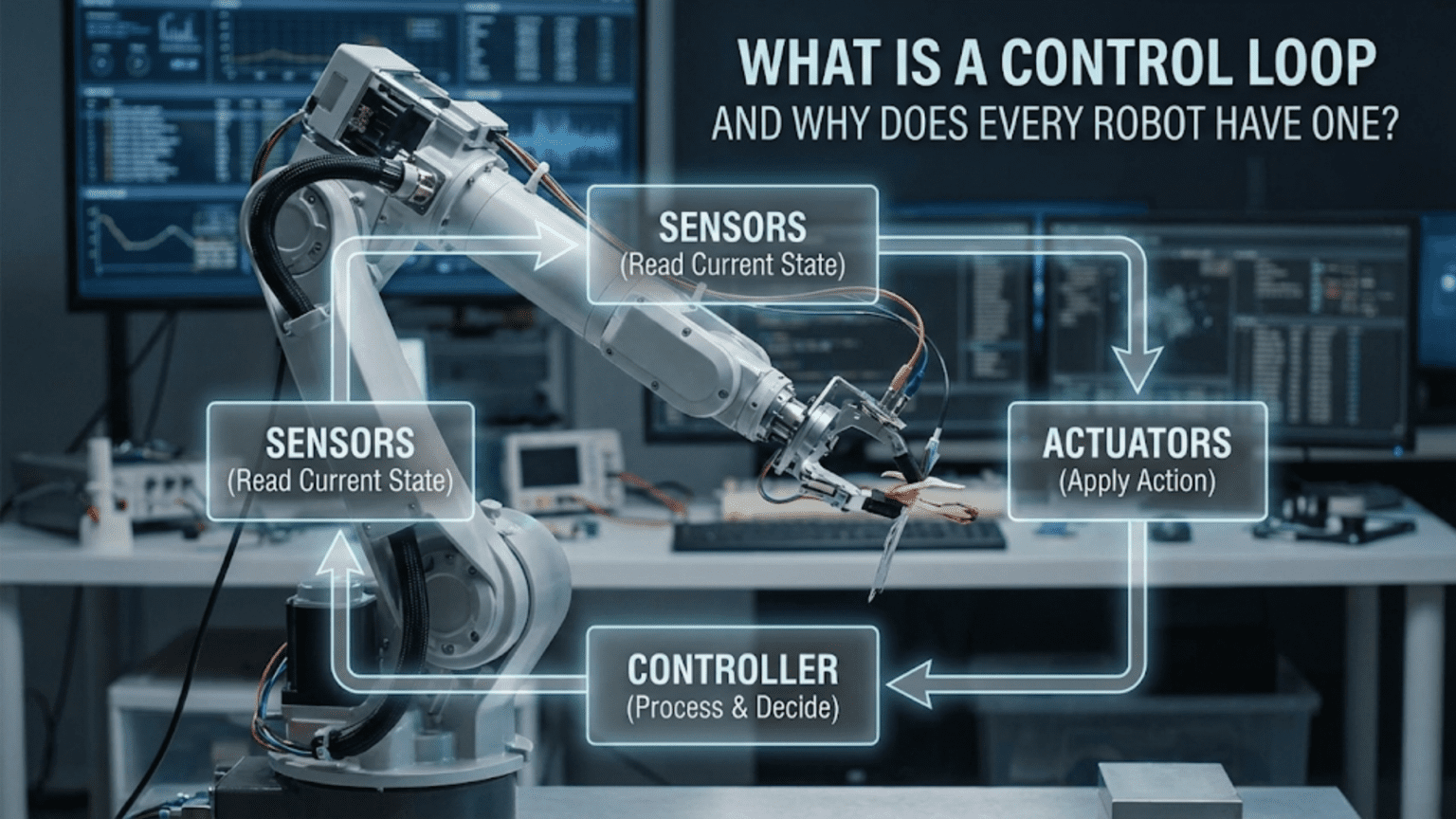
A control loop is a continuous cycle where a robot measures its current state through sensors, compares this measurement to a desired goal, calculates the difference (error), and adjusts its actions to minimize that error—repeating this process hundreds or thousands of times per second to maintain accurate, responsive behavior. Every robot uses control loops because they enable autonomous operation, compensate for disturbances, correct errors, and adapt to changing conditions without human intervention.
Your robot is meticulously following a black line on the floor, smoothly adjusting its path to stay centered despite slight variations in line width, floor texture, and ambient lighting. Or perhaps it’s maintaining a precise distance from a wall, neither drifting closer nor farther away as it navigates a corridor. Maybe it’s holding a robotic arm at exactly the position you commanded, resisting gravity and maintaining stability even when you place objects in its gripper. In every case, something remarkable is happening beneath the surface: your robot is continuously measuring, comparing, deciding, and adjusting—hundreds or thousands of times every second—in an endless cycle called a control loop.
Control loops represent the fundamental difference between a machine that blindly executes commands and a robot that intelligently responds to its environment. Without control loops, your line-following robot would drive straight off the path at the first curve. Your wall-following robot would crash at the first irregularity. Your robotic arm would droop under load and drift from its target position. Control loops are what transform simple mechanical systems into responsive, adaptive, autonomous robots.
Understanding control loops is essential for anyone progressing beyond the most basic robots. This concept appears everywhere in robotics—from the simplest line follower to the most sophisticated autonomous vehicle. Whether you’re consciously implementing control algorithms or using libraries that hide the details, control loops are running continuously, making thousands of tiny adjustments that keep your robot performing as intended. This article explains what control loops are, why they’re necessary, how they work, and most importantly, how to implement them in your own robots.
The Problem Control Loops Solve: Open-Loop Limitations
Before understanding control loops, you need to appreciate the problem they solve. Consider what happens when you command a robot without feedback—this is called open-loop control.
Open-Loop Control: Commanding Without Feedback
In open-loop control, you send a command to an actuator (motor, servo, etc.) and hope it does what you intended. For example, you might program:
// Open-loop motor control
digitalWrite(motorPin, HIGH);  // Turn motor on
delay(2000);                   // Run for 2 seconds
digitalWrite(motorPin, LOW); // Turn motor offYou’re commanding the motor to run for two seconds, assuming this makes your robot travel a specific distance. This works adequately under ideal conditions but fails when reality deviates from assumptions.
Why Open-Loop Fails in Real Conditions
Real-world factors that break open-loop assumptions include:
Variable loads: Your robot might carry different payloads. A motor that moves an empty robot 1 meter in 2 seconds might only move a loaded robot 0.7 meters in the same time. The open-loop command doesn’t know about the extra load.
Friction variations: Surfaces vary—carpet versus tile, clean versus dusty. The same motor command produces different speeds on different surfaces, making distance traveled unpredictable.
Battery voltage: As batteries drain, voltage drops, reducing motor speed. Early in operation, your two-second command might move the robot 1.2 meters. Near battery depletion, the same command might achieve only 0.8 meters.
Environmental disturbances: Wind, slopes, obstacles, and other forces push your robot off course. Open-loop control has no mechanism to detect or correct these disturbances.
Component tolerances: Two supposedly identical motors rarely perform identically due to manufacturing variations. Open-loop control can’t compensate for these differences.
The Missing Ingredient: Feedback
Open-loop control fails because it lacks feedback—information about what’s actually happening versus what you commanded. Without feedback, the robot blindly executes instructions regardless of results. This is like driving a car blindfolded, steering and accelerating based purely on memorized commands with no visual feedback about where you’re actually going.
Control loops solve this by closing the loop—adding sensors that measure actual results and algorithms that adjust commands based on those measurements. This transforms blind execution into intelligent, adaptive behavior.
Closed-Loop Control: The Feedback Solution
Closed-loop control adds feedback to create a continuous cycle of measuring, comparing, and correcting. This fundamental concept enables robots to achieve and maintain desired behaviors despite disturbances and uncertainties.
The Basic Control Loop Structure
Every control loop follows the same basic structure:
- Setpoint (Goal): Define the desired state (position, speed, distance, etc.)
- Measurement (Sensor): Measure the actual current state
- Error Calculation: Compute the difference between setpoint and measurement
- Control Action: Determine what to do to reduce the error
- Actuation: Apply the control action (adjust motor speed, change direction, etc.)
- Repeat: Continuously cycle through these steps
This creates a feedback loop where the output (robot’s actual state) feeds back into the input (control decision), allowing continuous self-correction.
A Simple Example: Distance Control
Suppose you want your robot to maintain exactly 20 cm from a wall using an ultrasonic distance sensor:
// Simple proportional control loop
const int targetDistance = 20;  // Setpoint: 20 cm
int currentDistance;             // Measured distance
int error;                       // Difference between target and actual
int motorSpeed;                  // Control output

void loop() {
  // Measure current state
  currentDistance = measureDistance();

  // Calculate error (positive if too far, negative if too close)
  error = targetDistance - currentDistance;

  // Calculate control action (move forward if too far, backward if too close)
  motorSpeed = error * 5;  // Proportional gain

  // Apply control action
  setMotorSpeed(motorSpeed);

  // Loop repeats continuously
}This simple control loop:
- Measures actual distance every cycle
- Calculates how far from target (error)
- Adjusts motor speed proportionally to error
- Larger errors produce stronger corrections
- Repeats continuously, making small adjustments
Even with disturbances (slopes, friction changes, battery drain), the robot continuously corrects toward the 20 cm target.
Why “Loop” Matters
The term “control loop” emphasizes the continuous, cyclical nature. This isn’t a one-time correction—it’s an endless cycle running dozens, hundreds, or even thousands of times per second. Each iteration makes a small adjustment based on current conditions, allowing the robot to continuously adapt to changing circumstances.
The loop frequency (how many times per second it executes) is critical:
- Too slow: Robot responds sluggishly, may oscillate or crash
- Too fast: May respond too aggressively or waste computational resources
- Just right: Smooth, stable control with minimal overshoot
Typical control loop frequencies range from 10 Hz (10 times per second) for slow systems to 1000 Hz (1000 times per second) for fast, precise control.
Types of Control Loops: From Simple to Sophisticated
Control loops range from extremely simple algorithms to complex adaptive systems. Understanding the progression helps you select appropriate approaches for your robots.
On-Off Control: The Simplest Loop
On-off control (also called bang-bang control) uses only two states: fully on or fully off.
Example: Temperature control
float currentTemp = readTemperature();
float targetTemp = 25.0;

if (currentTemp < targetTemp) {
  turnHeaterOn();    // Too cold, heat fully
} else {
  turnHeaterOff();   // Warm enough, heat off
}Advantages:
- Extremely simple to implement
- Requires minimal computation
- Works for many non-critical applications
Disadvantages:
- Oscillates around setpoint (overshoots, then undershoots repeatedly)
- Inefficient (wastes energy with full-power corrections)
- Mechanical wear from constant switching
- Poor precision
Best for: Simple, non-critical applications where oscillation is acceptable (thermostats, basic obstacle avoidance).
Proportional Control: Graduated Response
Proportional control adjusts the control action in proportion to the error size. Large errors produce strong corrections; small errors produce gentle corrections.
Formula: Control Output = Kp × Error
Where Kp is the proportional gain constant.
Example: Line following
const float Kp = 0.8;          // Proportional gain
int linePosition;              // Sensor reading (-100 to +100)
int targetPosition = 0;        // Goal: centered on line
int error;
int steeringCorrection;

void loop() {
  linePosition = readLineSensor();
  error = targetPosition - linePosition;
  steeringCorrection = Kp * error;

  // Apply steering correction to motors
  leftMotor = baseSpeed + steeringCorrection;
  rightMotor = baseSpeed - steeringCorrection;

  setMotorSpeeds(leftMotor, rightMotor);
}Advantages:
- Smooth, graduated corrections
- Less oscillation than on-off
- Simple to implement and tune
- Works well for many applications
Disadvantages:
- Steady-state error (may not reach exact target)
- No compensation for integral effects
- Slow response to rapid changes
Best for: Line following, basic navigation, gentle corrections where perfect accuracy isn’t critical.
PID Control: The Industry Standard
PID (Proportional-Integral-Derivative) control combines three complementary correction methods to achieve fast, accurate, stable control.
The Three Components:
P (Proportional): Corrects based on current error
- Larger error → stronger correction
- Provides primary corrective force
I (Integral): Corrects based on accumulated error over time
- Eliminates steady-state error
- Compensates for constant disturbances (gravity, friction, wind)
- Accumulates past errors and adds correction
D (Derivative): Corrects based on rate of error change
- Predicts future error based on current trend
- Dampens oscillation
- Prevents overshoot
Formula: Control Output = (Kp × Error) + (Ki × ∫Error dt) + (Kd × dError/dt)
Example: Position control
float Kp = 2.0;
float Ki = 0.5;
float Kd = 1.0;

float error = 0;
float lastError = 0;
float errorSum = 0;
float errorRate = 0;

float targetPosition = 100;  // Goal position
float currentPosition;
float output;

void loop() {
  currentPosition = readEncoder();

  // Calculate error
  error = targetPosition - currentPosition;

  // Proportional term
  float P = Kp * error;

  // Integral term (accumulated error)
  errorSum += error;
  float I = Ki * errorSum;

  // Derivative term (rate of change)
  errorRate = error - lastError;
  float D = Kd * errorRate;

  // Combined PID output
  output = P + I + D;

  // Apply to motor
  setMotorSpeed(output);

  lastError = error;
  delay(10);  // Control loop runs at ~100 Hz
}Advantages:
- Fast response without excessive overshoot
- Eliminates steady-state error
- Handles disturbances well
- Industry-proven and well-understood
Disadvantages:
- More complex to implement than simpler methods
- Requires careful tuning of three parameters
- Can become unstable if poorly tuned
Best for: Precise position control, speed regulation, temperature control, any application requiring accuracy and stability.
Advanced Control Methods
Beyond PID, advanced methods include:
Fuzzy Logic Control: Uses linguistic rules (“if error is large and increasing, apply strong correction”) rather than mathematical formulas. Good for complex systems difficult to model mathematically.
Model Predictive Control: Predicts future system behavior and optimizes control actions accordingly. Computationally intensive but excellent for complex multi-variable systems.
Adaptive Control: Automatically adjusts control parameters based on changing system characteristics. Handles systems with significant time-varying behavior.
Neural Network Control: Uses trained neural networks to generate control actions. Excellent for highly nonlinear or difficult-to-model systems.
For most hobby and educational robotics, PID control provides the best balance of performance and complexity. Advanced methods become relevant in professional applications or research projects.
Implementing Your First Control Loop: Practical Example
Let’s build a complete working control loop for a common robotics task: maintaining a constant distance from a wall while driving parallel to it.
Hardware Requirements
- Arduino (Uno or compatible)
- Ultrasonic distance sensor (HC-SR04 or similar)
- Two DC motors with driver (L298N or similar)
- Chassis with wheels
- Battery (appropriate for motors)
The Control Objective
Maintain exactly 15 cm distance from a wall while moving forward at constant speed. The control loop adjusts steering to keep distance constant despite:
- Wall irregularities
- Floor surface variations
- Motor speed differences
- Battery voltage changes
Complete Implementation
// Pin definitions
const int trigPin = 9;
const int echoPin = 10;
const int motorLeftFwd = 3;
const int motorLeftBwd = 4;
const int motorRightFwd = 5;
const int motorRightBwd = 6;
const int motorLeftPWM = 7;
const int motorRightPWM = 8;

// Control parameters
const float targetDistance = 15.0;  // Desired distance in cm
const int baseSpeed = 150;          // Base forward speed (0-255)
const float Kp = 3.0;               // Proportional gain

// Variables
float currentDistance;
float error;
int steeringCorrection;
int leftSpeed;
int rightSpeed;

void setup() {
  // Initialize pins
  pinMode(trigPin, OUTPUT);
  pinMode(echoPin, INPUT);
  pinMode(motorLeftFwd, OUTPUT);
  pinMode(motorLeftBwd, OUTPUT);
  pinMode(motorRightFwd, OUTPUT);
  pinMode(motorRightBwd, OUTPUT);
  pinMode(motorLeftPWM, OUTPUT);
  pinMode(motorRightPWM, OUTPUT);

  // Initialize serial for debugging
  Serial.begin(9600);
  Serial.println("Wall-following control loop started");
}

void loop() {
  // MEASURE: Get current distance from wall
  currentDistance = measureDistance();

  // CALCULATE ERROR: How far from target?
  error = targetDistance - currentDistance;
  // Positive error: too far from wall, need to turn toward it
  // Negative error: too close to wall, need to turn away

  // COMPUTE CONTROL ACTION: Proportional steering correction
  steeringCorrection = Kp * error;

  // Limit correction to prevent extreme steering
  steeringCorrection = constrain(steeringCorrection, -100, 100);

  // APPLY CONTROL: Adjust motor speeds
  // If error is positive (too far), increase right speed, decrease left (turn right)
  // If error is negative (too close), increase left speed, decrease right (turn left)
  leftSpeed = baseSpeed - steeringCorrection;
  rightSpeed = baseSpeed + steeringCorrection;

  // Ensure speeds stay in valid range
  leftSpeed = constrain(leftSpeed, 0, 255);
  rightSpeed = constrain(rightSpeed, 0, 255);

  // Set motor directions (both forward)
  digitalWrite(motorLeftFwd, HIGH);
  digitalWrite(motorLeftBwd, LOW);
  digitalWrite(motorRightFwd, HIGH);
  digitalWrite(motorRightBwd, LOW);

  // Set motor speeds
  analogWrite(motorLeftPWM, leftSpeed);
  analogWrite(motorRightPWM, rightSpeed);

  // Debug output
  Serial.print("Distance: ");
  Serial.print(currentDistance);
  Serial.print(" cm, Error: ");
  Serial.print(error);
  Serial.print(", Left: ");
  Serial.print(leftSpeed);
  Serial.print(", Right: ");
  Serial.println(rightSpeed);

  // Control loop delay (determines loop frequency)
  delay(50);  // 20 Hz control loop
}

float measureDistance() {
  // Trigger ultrasonic pulse
  digitalWrite(trigPin, LOW);
  delayMicroseconds(2);
  digitalWrite(trigPin, HIGH);
  delayMicroseconds(10);
  digitalWrite(trigPin, LOW);

  // Measure echo duration
  long duration = pulseIn(echoPin, HIGH, 30000);  // Timeout after 30ms

  // Convert to distance (speed of sound = 343 m/s)
  float distance = duration * 0.0343 / 2.0;

  // Handle timeout or out-of-range readings
  if (distance == 0 || distance > 200) {
    distance = 200;  // Return max range if no valid reading
  }

  return distance;
}How This Control Loop Works
Step 1: Measurement The measureDistance() function triggers the ultrasonic sensor and calculates distance to the wall.
Step 2: Error Calculation Error = target (15 cm) – actual distance. If the robot is 18 cm from the wall, error = -3 cm (too far).
Step 3: Control Calculation Steering correction = Kp × error = 3.0 × (-3) = -9. This negative value means turn toward the wall.
Step 4: Actuation Left motor: 150 – (-9) = 159 Right motor: 150 + (-9) = 141 The right motor slows down relative to the left, causing the robot to turn right (toward the wall).
Step 5: Repeat Loop executes every 50ms (20 times per second), continuously adjusting steering to maintain 15 cm distance.
Tuning the Control Loop
The Kp value (3.0) determines how aggressively the robot corrects. Tuning involves finding the optimal value:
Kp too low (e.g., 0.5):
- Slow, gentle corrections
- Robot drifts far from target before correcting
- Weak response to disturbances
- Stable but imprecise
Kp too high (e.g., 10.0):
- Strong, aggressive corrections
- Robot oscillates (swerves back and forth)
- Overshoots target repeatedly
- Unstable, jerky motion
Kp optimal (around 2.0-4.0 for this example):
- Quick but smooth corrections
- Minimal overshoot
- Stable, precise tracking
- Good disturbance rejection
Tuning procedure:
- Start with Kp = 1.0
- Increase gradually while testing
- Note when oscillation begins
- Reduce to about 60% of oscillation threshold
- Test in various conditions and adjust as needed
Real-World Control Loop Applications in Robotics
Control loops appear throughout robotics in diverse applications. Understanding these examples helps you recognize when and how to implement control loops in your own projects.
Line Following: Position Control
Goal: Keep robot centered on a line.
Sensor: Infrared line sensor array measuring position relative to line center.
Control Loop:
// Simplified line-following control loop
int linePosition = readLineSensor();  // -100 (far left) to +100 (far right)
int targetPosition = 0;                // Center of line
int error = targetPosition - linePosition;

int baseSpeed = 120;
int Kp = 2;
int correction = Kp * error;

int leftMotor = baseSpeed + correction;
int rightMotor = baseSpeed - correction;

setMotors(leftMotor, rightMotor);Why it works: Error represents deviation from line center. Positive error (line to the left) increases left motor speed and decreases right motor speed, turning the robot left back toward the line. The control loop runs continuously at high frequency, making tiny steering adjustments that keep the robot on track.
Speed Control: Velocity Regulation
Goal: Maintain constant motor speed despite varying load or battery voltage.
Sensor: Encoder measuring actual motor speed (RPM).
Control Loop:
// Motor speed control with PI controller
float targetRPM = 100.0;
float currentRPM = readEncoder();
float error = targetRPM - currentRPM;

static float errorSum = 0;
errorSum += error;

float Kp = 0.5;
float Ki = 0.1;

float output = (Kp * error) + (Ki * errorSum);
setMotorPWM(output);Why it works: If the motor slows down (uphill, added load), error becomes positive, increasing PWM to compensate. The integral term accumulates small persistent errors, ensuring the motor eventually reaches exact target speed even with constant load.
Balance Control: Inverted Pendulum
Goal: Keep a two-wheeled robot upright (like a Segway).
Sensor: IMU (gyroscope and accelerometer) measuring tilt angle and rate.
Control Loop:
// Simplified balance control (PD controller)
float targetAngle = 0.0;  // Vertical
float currentAngle = readIMU();
float error = targetAngle - currentAngle;

static float lastError = 0;
float errorRate = error - lastError;

float Kp = 50.0;  // Strong proportional for fast correction
float Kd = 5.0;   // Derivative to prevent oscillation

float motorPower = (Kp * error) + (Kd * errorRate);
setMotors(motorPower, motorPower);  // Both motors same direction

lastError = error;Why it works: Tilt forward creates positive error, driving motors forward to move the base under the top, correcting the tilt. The derivative term prevents overcorrection that would cause oscillation. This control loop must run very fast (100-1000 Hz) because balance is dynamically unstable.
Temperature Control: Environmental Regulation
Goal: Maintain electronics at safe operating temperature.
Sensor: Temperature sensor (thermistor, thermocouple, etc.).
Control Loop:
// Temperature control with PID
float targetTemp = 25.0;
float currentTemp = readTemperature();
float error = targetTemp - currentTemp;

static float errorSum = 0;
static float lastError = 0;

errorSum += error;
float errorRate = error - lastError;

float Kp = 5.0;
float Ki = 0.2;
float Kd = 1.0;

float fanSpeed = (Kp * error) + (Ki * errorSum) + (Kd * errorRate);
fanSpeed = constrain(fanSpeed, 0, 255);

setFanPWM(fanSpeed);
lastError = error;Why it works: Temperature rises above target, creating negative error (target – current < 0), which increases fan speed. Integral term ensures precise temperature maintenance. Derivative term prevents overshoot that would waste energy cycling the fan.
Gripper Force Control: Tactile Feedback
Goal: Grip objects with just enough force—not too loose (drops object), not too tight (damages object).
Sensor: Force sensor in gripper measuring grip pressure.
Control Loop:
// Force control with PI controller
float targetForce = 5.0;  // Newtons
float currentForce = readForceSensor();
float error = targetForce - currentForce;

static float errorSum = 0;
errorSum += error;

float Kp = 10.0;
float Ki = 2.0;

float gripperPower = (Kp * error) + (Ki * errorSum);
setGripperServo(gripperPower);Why it works: If force is too low (loose grip), positive error increases servo power, tightening grip. If force exceeds target (too tight), negative error decreases servo power, loosening slightly. The integral term ensures force converges to exact target.
Common Control Loop Problems and Solutions
Even well-designed control loops can exhibit problems. Recognizing these issues and knowing how to fix them is essential for successful implementation.
Problem: Oscillation Around Setpoint
Symptoms: Output swings back and forth across the target; system never settles.
Example: Line-following robot swerves left and right excessively rather than smoothly following the line.
Causes:
- Proportional gain (Kp) too high
- Derivative gain (Kd) too low (insufficient damping)
- Control loop running too slowly
- Sensor noise amplified by high gains
Solutions:
- Reduce Kp: Lower proportional gain until oscillation stops
- Add or increase Kd: Derivative term dampens oscillation
- Increase loop frequency: Faster control loop responds better
- Filter sensor readings: Average multiple readings to reduce noise
Problem: Steady-State Error
Symptoms: Output settles near but not at the target; constant offset remains.
Example: Wall-following robot consistently maintains 18 cm instead of target 15 cm.
Causes:
- Missing or insufficient integral term (Ki)
- Constant disturbance (gravity, friction) not compensated
- Proportional-only control reaches equilibrium before target
Solutions:
- Add integral term: Ki accumulates error and eliminates offset
- Increase Ki: If integral term exists but too small
- Check for mechanical issues: Binding, friction, or other resistance might prevent reaching target
Problem: Overshoot
Symptoms: Output exceeds target, then corrects, possibly oscillating.
Example: Robot approaching wall target overshoots, gets too close, then backs away repeatedly.
Causes:
- Kp too high (aggressive correction)
- Kd too low (insufficient prediction/damping)
- Control loop delay causes corrections to lag
Solutions:
- Reduce Kp: Gentler approach to target
- Increase Kd: Derivative term predicts and prevents overshoot
- Increase loop frequency: Faster response prevents lag-induced overshoot
Problem: Slow Response
Symptoms: System takes too long to reach target; sluggish corrections.
Example: Line-following robot drifts far from line before slowly correcting.
Causes:
- Kp too low (weak corrections)
- Control loop running too slowly
- Actuators underpowered for application
- Excessive filtering or averaging reducing responsiveness
Solutions:
- Increase Kp: Stronger corrections respond faster
- Increase loop frequency: Faster updates enable quicker response
- Reduce filtering: Balance noise rejection against responsiveness
- Verify actuator capability: Ensure motors/servos can deliver required performance
Problem: Integral Windup
Symptoms: Large overshoot when setpoint changes or disturbances clear; delayed response.
Example: Temperature controller overshoots dramatically when heater turns on after being saturated at maximum.
Causes:
- Integral term accumulates large value during saturation
- When saturation ends, accumulated integral drives huge overshoot
Solutions:
- Limit integral accumulation: Clamp errorSum to reasonable range
- Reset integral on saturation: If output saturates, stop accumulating or reduce errorSum
- Use anti-windup techniques: Sophisticated methods that prevent accumulation during saturation
// Anti-windup: limit integral accumulation
errorSum += error;
errorSum = constrain(errorSum, -1000, 1000); // Prevent excessive accumulationProblem: Noise Amplification
Symptoms: Jittery, unstable output; excessive corrections to sensor noise.
Example: Distance sensor noise causes constant unnecessary motor adjustments.
Causes:
- High derivative gain amplifies sensor noise
- Unfiltered noisy sensor readings
- Quantization in low-resolution sensors
Solutions:
- Filter sensor readings: Moving average, low-pass filter, or median filter
- Reduce Kd: Lower derivative gain
- Improve sensor quality: Better sensors with less noise
- Increase measurement resolution: Higher-resolution sensors provide smoother readings
// Simple moving average filter
const int numReadings = 5;
float readings[numReadings];
int readIndex = 0;
float total = 0;

void loop() {
  // Subtract old reading
  total -= readings[readIndex];

  // Add new reading
  readings[readIndex] = readSensor();
  total += readings[readIndex];

  // Advance index
  readIndex = (readIndex + 1) % numReadings;

  // Calculate average
  float filteredValue = total / numReadings;

  // Use filteredValue in control loop
}Comparison Table: Control Loop Types
| Control Type | Complexity | Accuracy | Responsiveness | Stability | Best Applications | Limitations |
|---|---|---|---|---|---|---|
| On-Off | Very Low | Poor | Fast | Poor (oscillates) | Thermostats, simple obstacle avoidance | Oscillation, inefficiency, poor precision |
| Proportional (P) | Low | Good | Fast | Good | Line following, basic navigation | Steady-state error, no disturbance compensation |
| Proportional-Integral (PI) | Moderate | Excellent | Moderate | Good | Speed control, temperature control | Can overshoot, requires tuning |
| Proportional-Derivative (PD) | Moderate | Good | Very Fast | Excellent | Balance control, high-speed systems | No steady-state error elimination |
| PID | Moderate-High | Excellent | Excellent | Excellent | Most robotics applications | Requires careful tuning, can be complex |
| Fuzzy Logic | High | Good | Good | Good | Complex or difficult-to-model systems | Requires expert knowledge, less predictable |
| Model Predictive | Very High | Excellent | Excellent | Excellent | Advanced robotics, multi-variable systems | High computational cost |
Best Practices for Control Loop Implementation
Successful control loop implementation requires more than just understanding the theory. These practical guidelines help you create reliable, well-performing systems.
Start Simple, Add Complexity as Needed
Begin with the simplest control that might work:
- Try proportional-only (P) control first
- Add integral (I) if steady-state error is problematic
- Add derivative (D) if oscillation or overshoot occurs
- Only use advanced methods if PID proves insufficient
Many robotics applications work perfectly with simple P or PI control. Don’t add unnecessary complexity.
Tune One Parameter at a Time
When adjusting PID parameters:
- Set Ki and Kd to zero, tune Kp first
- Once Kp gives acceptable response, add Ki if needed
- Finally add Kd if damping is required
- Make small adjustments and test after each change
Tuning procedure:
- Kp: Start at 1, double until oscillation begins, then reduce to 60-70% of that value
- Ki: Start at Kp/10, increase slowly until steady-state error eliminates
- Kd: Start at Kp/10, increase slowly until overshoot reduces without adding noise sensitivity
Choose Appropriate Loop Frequency
Control loop frequency depends on system dynamics:
- Slow systems (temperature): 1-10 Hz
- Moderate systems (position, distance): 10-100 Hz
- Fast systems (balance, high-speed motion): 100-1000 Hz
Too slow: Poor performance, instability Too fast: Wasted computation, noise amplification
Match frequency to system response time—about 10-20 times faster than the system’s natural response.
Implement Safety Limits
Always constrain outputs to safe, physically achievable ranges:
// Limit motor speeds
leftSpeed = constrain(leftSpeed, -255, 255);
rightSpeed = constrain(rightSpeed, -255, 255);

// Limit servo positions
servoAngle = constrain(servoAngle, 0, 180);

// Limit integral accumulation (prevent windup)
errorSum = constrain(errorSum, -1000, 1000);Safety limits prevent:
- Commanding impossible actions
- Integral windup
- Damage to hardware from excessive commands
- Erratic behavior from calculation errors
Add Diagnostic Outputs
Debugging control loops requires visibility into internal state:
// Print diagnostic information
Serial.print("Setpoint: ");
Serial.print(setpoint);
Serial.print(", Actual: ");
Serial.print(actual);
Serial.print(", Error: ");
Serial.print(error);
Serial.print(", P: ");
Serial.print(P_term);
Serial.print(", I: ");
Serial.print(I_term);
Serial.print(", D: ");
Serial.print(D_term);
Serial.print(", Output: ");
Serial.println(output);This reveals:
- Whether sensor readings make sense
- If error calculation is correct
- How each term contributes to output
- Whether output is saturating
Plotting these values over time (using Serial Plotter or external tools) provides even better insight into control loop behavior.
Test in Controlled Conditions First
Before testing in real operational scenarios:
- Test on bench without full load
- Verify sensor readings are reasonable
- Check that control actions move in correct direction
- Gradually increase difficulty (add load, increase speed, etc.)
- Only deploy in real conditions after bench testing succeeds
This progressive approach isolates problems and prevents damage from poorly tuned control loops.
Conclusion: Control Loops as Robot Intelligence
Control loops transform machines into robots. Without them, you have mechanical systems that blindly execute programmed commands, failing whenever reality deviates from assumptions. With control loops, you have intelligent systems that measure their environment, evaluate their performance, and continuously adapt their behavior to achieve goals despite disturbances and uncertainties.
Every successful robot—from the simplest line follower to sophisticated autonomous vehicles—relies on control loops. The specific implementation varies (simple proportional control versus advanced adaptive algorithms), but the fundamental concept remains constant: measure, compare, correct, repeat. This continuous cycle of feedback and adjustment enables the autonomous, adaptive behavior that defines robotics.
The skills you develop implementing control loops transfer across all robotics domains. Whether you’re building hobby projects, competition robots, commercial products, or research platforms, you’ll repeatedly encounter situations requiring feedback control. The line-following robot you program today uses the same control concepts as professional systems costing thousands or millions of dollars—just scaled and refined for their specific applications.
Start by implementing simple control loops in your current projects. Add a proportional controller to your line follower instead of simple if-then logic. Implement speed control for your motors rather than running them at fixed PWM values. Add distance maintenance to your obstacle-avoiding robot. Each implementation teaches lessons about sensor noise, tuning, stability, and the difference between theory and practice.
As you gain experience, you’ll develop intuition for control loop design. You’ll recognize when a system needs more aggressive control (higher Kp) versus more damping (higher Kd). You’ll know when integral action is necessary versus when it causes problems. You’ll understand how loop frequency affects performance and stability. This intuition, combined with systematic tuning procedures, allows you to implement effective control loops efficiently rather than through trial and error.
Most importantly, embrace the iterative nature of control loop development. Your first implementation probably won’t work perfectly—expect to tune, adjust, debug, and refine. This is normal and expected. Professional control engineers spend significant time tuning systems even with sophisticated tools and deep understanding. As a learner, expect this process to take time, but know that each iteration teaches valuable lessons.
Control loops represent one of the most powerful concepts in robotics, enabling the autonomous, adaptive behavior that makes robots useful and interesting. Master this concept, and you’ll understand the invisible intelligence that makes robots work. Your robots will stop being slaves to programmed commands and start being adaptive systems that intelligently respond to their environment, achieving goals despite challenges and disturbances. That transformation—from blind execution to intelligent adaptation—is what control loops provide, and why every robot has one.