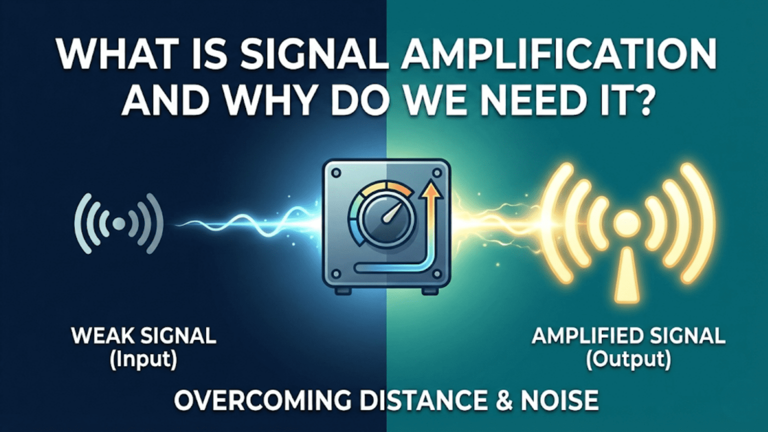
Signal amplification is the process of increasing the power, voltage, or current of an electrical signal using energy drawn from a power supply, enabling weak signals that are too small to be useful to drive outputs, be measured accurately, or be transmitted reliably. We need amplification because the physical world generates signals that are inherently tiny—a microphone converts sound to microvolts, a thermocouple produces millivolts per degree, a photodiode generates nanoamps of current—while the circuits that process, display, or transmit these signals typically require voltages of hundreds of millivolts to volts and currents of milliamps. Amplification bridges this gap, making the microscopic world of physical signals accessible to practical electronic systems.
Introduction: The Gap Between the World and Our Circuits
Every time you speak into a phone, your voice creates tiny pressure variations in the air. A microphone capsule converts those pressure variations into electrical signals — voltages that fluctuate in sympathy with the sound, rising and falling as your voice rises and falls. These electrical signals are faithful representations of your voice. They capture every nuance, every frequency, every subtle inflection.
But there is a problem. These signals are extraordinarily weak. A typical microphone produces signals of perhaps 1 millivolt — one thousandth of a volt — at moderate speaking volume. The circuitry that processes voice signals — analog-to-digital converters, radio transmitters, speakers — needs signals of hundreds of millivolts to volts. The gap between what the microphone produces and what the processing circuitry needs is enormous: a factor of 100 to 1000 or more.
This gap is not unique to microphones. It appears everywhere that electronics interfaces with the physical world. Thermocouples produce millivolts. Strain gauges produce microvolts. Photosensors produce nanoamps. Radio antennas receive signals measured in microvolts. Every sensor, every transducer, every physical measurement produces signals that are too small for direct use without amplification.
Signal amplification is the solution to this universal problem. An amplifier takes a weak input signal and produces a stronger output signal that faithfully represents the original — same waveform shape, same frequency content, same time relationships — but with greater voltage, current, or power. The extra energy comes from the power supply; the amplifier controls how that supply energy is released in proportion to the input signal, creating a magnified replica.
This article explores signal amplification comprehensively — what it actually is physically, why the world makes it necessary, the different ways gain can be expressed and measured, the types of amplifiers and what distinguishes them, the important practical concept of signal-to-noise ratio, and where amplification appears throughout the electronics you use every day.
Understanding amplification isn’t just academic. It’s the conceptual foundation for understanding why circuits are designed the way they are, why certain components must be placed close together, why power supply quality matters for sensitive measurements, and why the path from a physical phenomenon to a digital reading involves multiple carefully designed stages.
What Amplification Actually Does
The Physical Reality of Signal Amplification
Amplification is sometimes described as “making a signal bigger,” but this description misses the most important aspect: amplification adds energy to the signal from an external power supply.
This distinction matters deeply. A transformer can increase voltage without amplifying — but only at the cost of reduced current, so total power is unchanged (or reduced due to losses). Amplification genuinely increases power: the output signal has more power than the input signal. This additional power comes entirely from the DC power supply connected to the amplifier.
The amplifier as a controlled power supply: Think of an amplifier as a power supply whose output is controlled by the input signal. When the input signal goes positive, the amplifier draws more current from its supply and delivers more power to the output. When the input goes negative (or decreases), the amplifier reduces its output power accordingly. The result is that the output power mirrors the input waveform but at a much higher power level.
The transistor (or other active device) is the controlling element — it uses the tiny input signal to control the much larger current flowing from the power supply to the output.
Energy Conservation in Amplifiers
Amplifiers do not violate energy conservation. Total power out (signal + heat) always equals power in (from supply):
P_supply = P_output_signal + P_heat_dissipated
A perfect amplifier would convert all supply power into output signal power — efficiency of 100%. Real amplifiers have efficiencies ranging from below 1% (for Class A audio amplifiers running continuously) to over 90% (for Class D switching amplifiers). The difference is wasted as heat in the active devices.
Why this matters practically: High-power amplifiers — audio power amplifiers, RF transmitters, motor drives — dissipate significant heat. That heat must be managed through heatsinking, thermal design, and sometimes forced cooling. The efficiency class of an amplifier determines how much heat management is needed.
What Is Preserved During Amplification
Good amplification preserves the essential characteristics of the signal while increasing its power:
Preserved:
- Waveform shape (the signal looks the same, just bigger)
- Frequency content (the amplifier doesn’t add or remove frequencies)
- Timing relationships (the signal isn’t stretched or compressed in time, though small delays are introduced)
- Phase relationships (in ideal amplifiers; real amplifiers introduce phase shifts at frequency extremes)
Modified:
- Amplitude (voltage and/or current — this is the purpose)
- Power level (always increased; this is the definition)
- Noise (amplifiers add their own noise to the signal — unavoidable but minimized in good design)
- Distortion (perfect linearity is an ideal; real amplifiers introduce small nonlinearities)
Gain: Quantifying Amplification
Voltage Gain
Voltage gain (A_v) is the ratio of output voltage to input voltage:
A_v = V_out / V_in
Example: A microphone preamplifier takes a 2mV microphone signal and produces a 400mV output. A_v = 400mV / 2mV = 200
The amplifier provides a voltage gain of 200 — it multiplied the voltage by 200.
Voltage gain can also be less than 1 (attenuator), exactly 1 (buffer), or negative (inverting amplifier — output is flipped in phase relative to input).
Current Gain
Current gain (A_i) is the ratio of output current to input current:
A_i = I_out / I_in
Example: A transistor with base current of 10μA drives a collector current of 1mA. A_i = 1mA / 10μA = 100
In a transistor amplifier, this current gain (β or hFE) is the fundamental amplification mechanism.
Power Gain
Power gain (A_p) is the ratio of output power to input power:
A_p = P_out / P_in = (V_out × I_out) / (V_in × I_in)
Power gain relates to both voltage and current gain: A_p = A_v × A_i
Power gain is always positive (greater than 1 for a true amplifier), even when voltage gain is less than 1 (an impedance-matching amplifier can have high current gain and power gain despite unity voltage gain).
Decibels: The Logarithmic Scale for Gain
Gain expressed as a simple ratio (200×, 1000×) becomes unwieldy when dealing with the enormous range of amplifications encountered in practice — from 0.001 to 1,000,000 and beyond. Decibels (dB) compress this range into manageable numbers using logarithms.
Voltage gain in decibels: A_v(dB) = 20 × log₁₀(V_out / V_in)
Power gain in decibels: A_p(dB) = 10 × log₁₀(P_out / P_in)
Key decibel values to memorize:
| Voltage ratio | Power ratio | dB value |
|---|---|---|
| 1 (unity gain) | 1 | 0 dB |
| √2 ≈ 1.414 | 2 | +3 dB |
| 2 | 4 | +6 dB |
| 10 | 100 | +20 dB |
| 100 | 10,000 | +40 dB |
| 1000 | 1,000,000 | +60 dB |
| 0.5 | 0.25 | −6 dB |
| 0.1 | 0.01 | −20 dB |
Why decibels are convenient:
- Gains of cascaded amplifiers add in dB instead of multiplying: 20dB + 40dB + 20dB = 80dB total (versus 10 × 100 × 10 = 10,000 as a ratio)
- The ear perceives loudness logarithmically — decibels match human perception
- Frequency response plots (Bode plots) use dB on the vertical axis, making complex behaviors visible as simple slopes
Example: A three-stage amplifier with gains of 10, 50, and 20:
- As ratios: Total gain = 10 × 50 × 20 = 10,000
- In decibels: 20dB + 34dB + 26dB = 80dB
- Verification: 20 × log₁₀(10,000) = 80dB ✓
Bandwidth and the Gain-Bandwidth Trade-Off
Amplifiers don’t provide equal gain at all frequencies. Every amplifier has a bandwidth — a range of frequencies over which it amplifies effectively.
-3dB bandwidth: The standard definition of bandwidth is the frequency range between the points where gain drops to -3dB (approximately 70.7%) of the midband maximum. At the -3dB frequency, the amplifier delivers half the power of its peak.
Gain-bandwidth product (GBW): For many amplifier types, gain and bandwidth are linked by a constant:
Gain × Bandwidth = Constant (GBW)
Doubling the gain halves the bandwidth. This is an inherent property of many amplifier topologies.
Practical implication: A high-gain amplifier has narrower bandwidth. An audio amplifier that amplifies 20Hz–20kHz (20kHz bandwidth) can achieve much higher gain than an RF amplifier that must handle 88MHz–108MHz (20MHz bandwidth at much higher frequency).
Why We Need Amplification: The Signal Chain
The Concept of a Signal Chain
A signal chain is the sequence of stages a signal passes through from its source to its destination. Each stage performs a specific function — sensing, amplification, filtering, conversion, transmission, display. Understanding amplification requires understanding its role within this chain.
Typical signal chain:
Physical World → Sensor/Transducer → [Amplification] → Processing → OutputReal examples:
Audio recording: Sound → Microphone → Preamplifier → ADC → Digital Processing → DAC → Power Amplifier → Speaker
Temperature measurement: Temperature → Thermocouple → Instrumentation Amplifier → ADC → Microcontroller → Display
Medical ECG: Heart electrical activity → Electrodes → Differential Amplifier → High-pass filter → Notch filter (60Hz) → ADC → Display
Radio reception: RF signal (antenna) → LNA (Low-Noise Amplifier) → Mixer → IF Amplifier → Detector → Audio Amplifier → Speaker
In every case, amplification appears at or near the beginning of the signal chain — as close to the source as possible — to boost the weak signal before it gets buried in the noise of subsequent processing stages.
Why Amplify Early? The Noise Figure Argument
The critical principle: Noise added in early stages of a signal chain is amplified along with the signal through all subsequent stages. Noise added in later stages affects only the final output.
Mathematical illustration:
Signal chain with two stages, each with gain = 10 and noise floor = 1mV:
- Input signal: 1mV
- After Stage 1: Signal = 10mV, Noise = 1mV (from Stage 1 itself), SNR = 10
- After Stage 2: Signal = 100mV, Noise = 10mV (Stage 1 noise amplified) + 1mV (Stage 2 noise) = 11mV, SNR ≈ 9
Now suppose we add a poor-quality Stage 1 with 10mV of noise:
- After Stage 1: Signal = 10mV, Noise = 10mV, SNR = 1 (terrible!)
- After Stage 2: Signal = 100mV, Noise = 100mV + 1mV = 101mV, SNR ≈ 1 (still terrible)
The lesson: The first amplifier in a signal chain must be designed for minimum noise (low noise figure). All subsequent stages amplify whatever SNR the first stage established. No amount of perfect design in later stages recovers SNR lost at the input.
This is why low-noise amplifiers (LNAs) are given such attention in radio receivers, scientific instruments, and audio recording — they set the noise floor for the entire system.
Sensors and Transducers: Why Their Outputs Are Weak
Every physical sensing process has a fundamental limit on signal strength:
Microphones: Sound pressure → diaphragm motion → electrical signal (capacitive or electromagnetic). The mechanical-to-electrical conversion has low efficiency. Output: 1–10mV for typical speech levels.
Thermocouples: Temperature difference → Seebeck effect → voltage. Output: ~40μV per °C (for type K thermocouple). A 100°C temperature difference generates just 4mV.
Strain gauges: Mechanical deformation → resistance change → bridge voltage. Output: Typically 1–3mV per volt of excitation at full scale deflection. With 5V excitation: 5–15mV full scale.
Photodiodes: Photons → electron-hole pairs → current. Output: Nanoamps to microamps depending on illumination.
Piezoelectric sensors: Vibration/pressure → charge separation → voltage. Output: High voltage but extremely high impedance — can’t drive any load without buffering.
Antenna (radio): Electromagnetic field → induced EMF. Output: Microvolts to millivolts depending on field strength and antenna size.
All of these need amplification — often significant amplification — before their signals can be digitized, transmitted, or displayed.
Types of Amplifiers
By Signal Type
Voltage amplifiers: Primary purpose: increase voltage. Input and output both specified as voltages. Most common type discussed in educational contexts. Examples: op-amp inverting amplifier, common-emitter transistor amplifier.
Current amplifiers: Primary purpose: increase current. Input specified as current, output as current. Less common standalone; common as part of transimpedance amplifiers. Example: current mirror.
Transimpedance amplifiers (TIA): Convert current input to voltage output. Gain specified in ohms (V/A). Essential for photodiode and other current-source sensors. Example: op-amp with feedback resistor from output to inverting input.
Transconductance amplifiers: Convert voltage input to current output. Gain specified in siemens (A/V). Used in voltage-controlled current sources. Example: differential pair with tail current.
Power amplifiers: Deliver power to a load (speaker, motor, antenna). Gain often specified in watts per watt or dB. Efficiency and linearity are paramount concerns.
By Operating Class
The operating class describes how the active device is biased relative to the signal swing:
Class A: The active device conducts throughout the entire 360° of the input signal cycle. Output transistor always on. Excellent linearity (low distortion). Very low efficiency (25–30% theoretical maximum for resistive load). Used in high-fidelity audio preamplifiers, input stages.
Class B: Two complementary devices each handle one half-cycle (180°). Each device is off for the half-cycle it doesn’t handle. Efficiency up to 78.5% theoretical. Suffers from crossover distortion at the transition point between devices.
Class AB: A compromise between A and B. Both devices are biased slightly on, overlapping near the zero crossing. Reduces crossover distortion while maintaining reasonable efficiency (50–70%). Standard for most audio power amplifiers.
Class D: Switching amplifier. Active devices operate as switches (fully on or fully off), not linear devices. Audio signal encoded as pulse-width modulated square wave; low-pass filter at output recovers audio. Efficiency >90% possible. Now dominates consumer audio. Some high-frequency distortion but excellent for most uses.
Class C: Active device conducts for less than 180° of the cycle. Very high efficiency (>80%) but very high distortion — only used in tuned (resonant) RF transmitter circuits where the tank circuit reconstructs the sine wave.
By Function
Preamplifier (preamp): The first amplification stage, closest to the signal source. Designed for minimum noise and sufficient gain to establish a good SNR. Examples: microphone preamplifiers, phonograph preamplifiers, instrument preamplifiers.
Driver amplifier: Intermediate stage providing power gain to drive the final output stage. Bridges the gap between preamplifier output and power amplifier input impedance requirements.
Power amplifier: Final stage delivering power to the load — speaker, antenna, motor. High current output, designed for efficiency and thermal management.
Instrumentation amplifier: High input impedance, differential input, precise gain, excellent common-mode rejection. Used for measurement of small differential signals in noisy environments. Strain gauge bridges, ECG electrodes, thermocouples.
Operational amplifier (op-amp): General-purpose amplifier building block with very high gain (~100,000), high input impedance, low output impedance. Used with feedback networks to create precision amplifiers, filters, oscillators, comparators.
RF/Microwave amplifiers: Designed for radio frequencies from MHz to GHz. Key metrics: gain, noise figure, IP3 (linearity), output power, and stability. Used in radios, radar, cellular base stations.
Signal-to-Noise Ratio: The True Measure of Quality
What SNR Measures
Signal-to-noise ratio (SNR) is the ratio of the desired signal power to the background noise power:
SNR = P_signal / P_noise
Or in decibels: SNR(dB) = 10 × log₁₀(P_signal / P_noise) = 20 × log₁₀(V_signal / V_noise)
A higher SNR means the signal is cleaner, more reliable, and more accurately measurable.
Practical SNR levels:
| SNR | Perception / Application |
|---|---|
| 0 dB | Signal equals noise — unusable |
| 10 dB | Signal barely discernible |
| 20 dB | Poor quality; significant noise audible |
| 40 dB | Acceptable for speech communications |
| 60 dB | Good quality audio |
| 80 dB | Excellent; background noise inaudible in most situations |
| 96 dB | Theoretical maximum of 16-bit audio |
| 120 dB | Excellent measurement instrument grade |
Why Amplification Doesn’t Improve SNR
A critical insight: amplification amplifies signal and noise equally. If the noise floor of an amplifier is 1mV and the signal is 10mV (SNR = 10), amplifying by 10 gives 100mV signal and 10mV noise — SNR is still 10.
This means:
- You cannot recover lost SNR by adding more amplification
- The SNR of the first stage is (approximately) the SNR of the entire system
- The only way to improve SNR is to either increase the signal (better sensor, better coupling) or decrease the noise (lower-noise amplifier, narrower bandwidth, filtering)
Noise Figure: Rating Amplifier Noise Performance
Noise figure (NF) quantifies how much an amplifier degrades the SNR of the signal passing through it:
NF(dB) = SNR_in(dB) – SNR_out(dB)
An ideal, noiseless amplifier has NF = 0dB. All real amplifiers have NF > 0dB.
Typical noise figures:
| Amplifier type | Typical NF |
|---|---|
| High-quality audio preamp | 2–5 dB |
| Instrumentation amplifier | 1–10 dB |
| Cellular LNA | 0.5–2 dB |
| Satellite receiver LNA | 0.1–0.5 dB |
| Cheap consumer audio IC | 5–15 dB |
For the first amplifier in a chain, minimize NF. Later stages contribute progressively less to total system noise figure (Friis formula — each subsequent stage’s noise contribution is divided by the gain of all preceding stages).
Where Amplification Appears in Everyday Electronics
Your Smartphone
Microphone path: Microphone → MEMS microphone amplifier (integrated) → Codec ADC → DSP → Radio transmitter
Receiver path: Antenna → LNA → RF front-end → Baseband amplifier → ADC → DSP → Earpiece amplifier → Speaker
Camera: Image sensor → Pixel-level amplifier (each pixel has a built-in source follower) → Column amplifiers → Analog-to-digital converter
Your phone contains dozens of amplifiers performing different functions simultaneously.
Audio Systems
Vinyl record playback: Phono cartridge (0.5mV) → RIAA phono preamplifier (40dB gain + equalization) → Preamplifier → Power amplifier → Speaker
Professional microphone: Condenser mic (1mV) → Phantom-powered buffer → XLR cable → Mixing desk preamp → EQ → Level fader → Output amplifier → Recording/PA system
Hearing aid: Microphone (tiny, high-noise) → DSP preamplifier → DSP (noise reduction, frequency shaping) → Output amplifier → Receiver (miniature speaker in ear)
Medical Electronics
ECG (Electrocardiogram): Heart signal on skin surface: ~1mV, contaminated with 60Hz interference, motion artifacts, and muscle noise.
Required: Differential amplifier rejecting common-mode 60Hz, high-pass filter removing baseline wander, amplification of ~1000× to get 1V signal, notch filter for 60Hz rejection, isolation amplifier for patient safety.
Without careful amplification design, ECG is impossible — the signal is too small and too noisy for direct measurement.
Blood glucose sensor: Electrochemical reaction at electrode → current of nanoamps to microamps → transimpedance amplifier (converts current to voltage) → ADC → glucose reading
Scientific Instruments
Seismometer: Ground motion → velocity transducer → low-noise preamplifier → recording system. Detects earthquakes thousands of kilometers away; the signal amplification chain must be extraordinarily sensitive without adding noise.
Radio telescope: Antenna → cryogenically cooled LNA (cooled to near absolute zero to minimize thermal noise) → multiple amplification stages → spectrometer. Detects radio emissions from distant galaxies — signals at power levels of 10⁻²⁰ watts.
Scanning electron microscope: Secondary electron detector → electron multiplier → transimpedance amplifier → ADC → image. Signal from electron detector can be single electrons, requiring near-quantum-limit amplification.
Comparison Table: Amplifier Types and Applications
| Amplifier Type | Input | Output | Key Metric | Typical Gain | Primary Application |
|---|---|---|---|---|---|
| Voltage amplifier | Voltage | Voltage | A_v (V/V) | 2–10,000 | General signal amplification |
| Current amplifier | Current | Current | A_i (A/A) | 10–1000 | Transistor base-to-collector |
| Transimpedance | Current | Voltage | Z_T (Ω = V/A) | 1kΩ–100MΩ | Photodiodes, sensors |
| Transconductance | Voltage | Current | G_m (S = A/V) | 1mS–100mS | VCO, mixer inputs |
| Power amplifier | Low power | High power | Efficiency (%) | 10W–1000W | Speakers, RF transmitters |
| Instrumentation amp | Differential V | Single-ended V | CMRR, precision | 1–10,000 | Sensor bridges, medical |
| Low-noise amp (LNA) | Weak RF signal | Amplified RF | Noise figure (dB) | 10–30 dB | Radio receivers, radar |
| Operational amp (op-amp) | Differential V | Single V | Open-loop gain | 100,000+ (open) | Universal analog building block |
| Class A audio | Audio signal | Audio signal | THD, linearity | 20–40 dB | Audiophile preamps |
| Class D switching | Audio signal | Audio signal | Efficiency % | 20–50W | Consumer audio, mobile |
Practical Design Considerations
Gain Staging: Why Not Just Use One Big Amplifier?
A common beginner question: if you need a gain of 10,000, why use multiple amplifier stages instead of one stage with gain 10,000?
Reasons for multiple stages:
Stability: High-gain single stages are prone to oscillation. Parasitic feedback paths (capacitive coupling between output and input) become significant at high gain, causing the amplifier to self-oscillate. Multiple moderate-gain stages are inherently more stable.
Bandwidth: A single stage with gain 10,000 has very narrow bandwidth (gain-bandwidth product limited). Multiple stages each with gain of 30 dB (31.6×) can achieve the same total gain with much wider bandwidth — or equal bandwidth with lower noise figure per stage.
Dynamic range: Multiple stages allow filtering and processing between amplification steps. A high-pass filter after the first stage removes low-frequency noise before it gets further amplified. A limiting stage can be inserted to prevent overload of later stages.
Impedance matching: Each stage can be designed with optimal input and output impedance for its specific role in the chain.
The Importance of Power Supply Decoupling
Every amplifier’s power supply affects its noise and linearity. Supply voltage variations couple into the output signal through the power supply rejection ratio (PSRR — finite in all real amplifiers). A noisy power supply produces a noisy output, regardless of how good the amplifier design is.
This is why:
- Decoupling capacitors are required near every amplifier stage
- Linear voltage regulators (quieter than switching regulators) are preferred for sensitive analog circuits
- Separate supply rails for analog and digital circuits are standard in mixed-signal designs
- High-precision instruments use battery power or heavily filtered supplies to avoid contamination from AC power
Input and Output Impedance Matching
The maximum power transfer theorem: Maximum power transfers between a source and load when their impedances are equal (matched).
For voltage amplifiers (not matched): A voltage amplifier should have input impedance much higher than the source impedance and output impedance much lower than the load impedance. This is impedance bridging — the standard for audio and most signal amplifiers.
For RF amplifiers (matched): RF systems are designed for 50Ω impedance matching throughout. Mismatches cause reflections (standing waves) and power loss, particularly problematic at high frequencies.
The buffer (emitter follower or op-amp voltage follower): Transforms high-impedance sources to low-impedance outputs. Essential wherever a high-impedance sensor or amplifier output must drive a low-impedance load or long cable.
Conclusion: Amplification as the Foundation of Signal Processing
Signal amplification is the enabling technology behind virtually all practical electronics that interact with the physical world. Without it, sensors would be useless, communication would be impossible, and the digital revolution would have no window into physical reality.
The Key Insights
Amplification adds energy: The power in an amplified signal exceeds the power in the input signal. This additional power comes from the supply — the amplifier is a controlled power converter, not a free energy device.
Gain is multiplicative, decibels are additive: Whether expressed as a voltage ratio or in decibels, gain quantifies the amplification provided. Understanding both representations is essential for working with real signal chains.
SNR is set at the input: The first amplifier stage determines the noise floor of the entire system. Subsequent stages cannot recover SNR lost at the input. This makes low-noise design at the input stage the most critical design decision in sensitive systems.
Multiple stages beat one high-gain stage: Staging amplification in moderate-gain steps provides better stability, wider bandwidth, and more opportunity for intermediate filtering and processing.
Different applications, different amplifier types: Voltage amplifiers, transimpedance amplifiers, power amplifiers, instrumentation amplifiers — each optimized for its specific role in the signal chain.
The Path Forward
With a solid understanding of amplification concepts, the next steps in analog electronics become natural progressions:
- Op-amps: General-purpose amplifier building blocks that implement all these amplification functions with high precision and ease of design
- Filters: Frequency-selective circuits built from amplifier stages and passive components
- Feedback: The technique that stabilizes gain, reduces distortion, and extends bandwidth in real amplifiers
- Oscillators: Amplifiers with controlled positive feedback that generate signals
- Mixers and modulators: Non-linear amplifier applications for frequency conversion and signal modulation
The conceptual thread through all of these is the same: controlling larger amounts of energy using smaller signals, always faithfully representing the input in the output, always serving the fundamental goal of bringing the physical world’s microscopic signals into the realm of practical electronics.
Amplification is not a component or a circuit — it’s a fundamental capability, the bridge between the world as physics makes it and electronics as we design it.