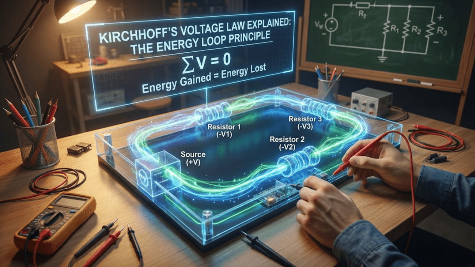
Kirchhoff’s Voltage Law Explained: The Energy Loop Principle

Kirchhoff’s Voltage Law (KVL) states that the algebraic sum of all voltages around any closed loop in a circuit equals zero, based on the principle of energy conservation. This means that as you trace a complete path through a circuit and return to your starting point, the total voltage rise (from power sources) must equal the total voltage drop (across components), making it an essential tool for analyzing series circuits and complex multi-loop networks.

Introduction: The Energy Journey Around a Circuit

Imagine hiking a circular trail that takes you up hills and down valleys, eventually returning you to your starting point. No matter how many ups and downs you experience along the way, one thing is certain: the total elevation gain must equal the total elevation loss. If you start and end at the same spot, your net change in elevation is zero.

This simple hiking analogy perfectly captures the essence of Kirchhoff’s Voltage Law (KVL). Just as elevation changes along a loop path must sum to zero, voltage changes around any closed loop in an electrical circuit must also sum to zero. This isn’t just a convenient mathematical trick—it’s a fundamental consequence of energy conservation in electrical systems.

Named after Gustav Kirchhoff, the same German physicist who gave us Kirchhoff’s Current Law (KCL), this principle was formulated in 1845 and remains one of the cornerstones of circuit analysis. While KCL focuses on what happens at junctions (where currents split or combine), KVL focuses on what happens around closed paths (where voltage rises and drops must balance).

Understanding KVL transforms circuit analysis from guesswork into systematic problem-solving. Whether you’re calculating voltage drops across resistors in a series circuit, analyzing a complex power supply with multiple voltage sources, designing sensor circuits, or troubleshooting why your circuit isn’t working as expected, KVL provides the mathematical framework you need.

In this comprehensive guide, we’ll explore every aspect of Kirchhoff’s Voltage Law: its theoretical foundation in energy conservation, how to identify loops and assign voltage polarities correctly, systematic methods for writing KVL equations, practical applications in real circuits, common mistakes to avoid, and how KVL combines with other circuit laws to enable complete circuit analysis.

By the end of this article, you’ll understand not just what KVL states, but why it must be true, and how to apply it confidently to solve real-world circuit problems. Let’s begin our journey around the voltage loop.

What is Kirchhoff’s Voltage Law?

The Basic Statement

Kirchhoff’s Voltage Law can be expressed in several equivalent ways:

Formal statement: The algebraic sum of all voltages around any closed loop in a circuit equals zero.

Practical statement: The sum of all voltage rises around a loop equals the sum of all voltage drops around that loop.

Mathematical statement: ΣV = 0 around any closed loop, where voltage rises are positive and voltage drops are negative (or vice versa).

The symbol Σ (sigma) means “sum of,” so ΣV means “the sum of all voltages around the loop.”

Understanding Voltage in Circuits

Before diving deeper into KVL, let’s ensure we understand what voltage actually represents:

Voltage is electrical potential difference: Just as gravitational potential energy depends on height, electrical potential energy depends on voltage. Voltage is the energy difference per unit charge between two points.

Voltage is always relative: You can’t talk about “the voltage at a point” without specifying what you’re measuring relative to. We always measure voltage between two points (a voltage difference).

Voltage represents energy per charge: One volt means one joule of energy per coulomb of charge (1V = 1J/C). When charge moves through a voltage difference, energy is transferred.

Voltage sources add energy: Batteries, power supplies, and generators increase the electrical potential energy of charges passing through them. We call this a “voltage rise.”

Passive components drop voltage: Resistors, LEDs, motors, and other loads decrease the electrical potential energy of charges, converting it to other forms (heat, light, motion). We call this a “voltage drop.”

What is a Loop?

Just as KCL requires understanding nodes, KVL requires understanding loops:

Definition: A loop is any closed path through a circuit—a route that starts at a point, travels through circuit elements, and returns to the starting point without retracing any segment.

Simple loop: A basic circuit with one voltage source and one or more components in series forms a single loop.

Multiple loops: Complex circuits can have many different loops. You can trace different paths through the same circuit, creating different loops.

Independent loops: Some loops share components with other loops, while truly independent loops (meshes) share no interior paths. For circuit analysis, independent loops are most useful.

Direction doesn’t matter: You can trace a loop clockwise or counterclockwise—KVL works either way. What matters is consistency in how you assign voltage polarities.

The Physical Basis: Conservation of Energy

KVL isn’t arbitrary—it’s a direct consequence of energy conservation:

Energy in equals energy out: In a complete loop, any energy added to charges (by voltage sources) must equal the energy removed from charges (by loads). Otherwise, charges would gain or lose energy during each loop, creating a perpetual motion machine—physically impossible.

Electric field is conservative: The work done by electric forces on a charge moving around any closed path is zero. This is a fundamental property of electrostatic fields.

Path independence: The voltage difference between two points is the same regardless of what path you take between them (in DC circuits). This means completing a loop—traveling from point A back to point A—must result in zero net voltage change.

The consequence: Since energy is conserved, and voltage represents energy per unit charge, the sum of all voltage changes around a loop must be zero. This is KVL.

Analogy: Just as gravitational potential energy change around a closed path is zero (you end at the same elevation you started), electrical potential energy change around a closed circuit path is zero.

Sign Conventions

Correctly assigning signs to voltages is crucial for applying KVL. Here’s the systematic approach:

Method 1: Rise vs. Drop

• Voltage rises (sources): Assign positive (+) sign
• Voltage drops (loads): Assign negative (-) sign
• Then: ΣV = 0

Method 2: Polarity and Loop Direction

• Choose a loop direction (clockwise or counterclockwise)
• For each component, note its polarity (+ and – terminals)
• If traveling + to -, voltage is negative (drop)
• If traveling – to +, voltage is positive (rise)
• Then: ΣV = 0

Both methods work. Method 2 is more systematic and less prone to error in complex circuits.

Critical point: The polarity markings (+ and -) on components indicate which terminal has higher potential. This is independent of your chosen loop direction.

A Simple Example

Consider a basic circuit:

• 9V battery (positive terminal on top)
• Two resistors in series: R₁ = 300Ω, R₂ = 600Ω
• Current flows: 10 mA

Applying KVL clockwise starting from battery negative terminal:

Step 1: Identify voltages around the loop

• Battery: Travel from – to +, this is a voltage rise = +9V
• R₁: Current flows top to bottom, so top is +, bottom is –
  • Voltage across R₁: V₁ = I × R₁ = 0.01A × 300Ω = 3V
  • Traveling top to bottom (+ to -), this is a drop = -3V
• R₂: Current flows top to bottom, top is +, bottom is –
  • Voltage across R₂: V₂ = I × R₂ = 0.01A × 600Ω = 6V
  • Traveling top to bottom (+ to -), this is a drop = -6V

Step 2: Apply KVL ΣV = 0 +9V – 3V – 6V = 0 0 = 0 ✓

The voltages balance! The 9V rise from the battery equals the 9V total drop across the resistors (3V + 6V).

The Mathematical Foundation of KVL

The General KVL Equation

For a loop containing n components (voltage sources and voltage drops):

ΣV = V₁ + V₂ + V₃ + … + Vₙ = 0

Where each voltage gets a positive or negative sign based on the chosen sign convention.

Equivalently: ΣV_rises = ΣV_drops

The total voltage supplied by sources equals the total voltage consumed by loads.

In summation notation: Σᵢ₌₁ⁿ Vᵢ = 0

This is the most compact mathematical form.

KVL for Multiple Loops

Circuits with multiple loops require multiple KVL equations:

For a circuit with n independent loops: You can write n independent KVL equations.

Independent loops (meshes): These are loops that don’t share interior paths—each contains at least one component not in any other loop.

Example: A circuit with two voltage sources and three resistors arranged in a ladder network has two independent loops.

The system of equations: Multiple KVL equations (plus Ohm’s Law relationships) create a system you can solve for unknown voltages and currents.

Combining KVL with Ohm’s Law

KVL becomes most powerful when combined with Ohm’s Law:

For resistors: V = I × R If you know current and resistance, you can find voltage drop. If you know voltage and resistance, you can find current.

In a loop: Express all resistor voltages as (I × R) terms, then apply KVL.

Example: Loop with battery (V_battery) and three resistors (R₁, R₂, R₃) in series:

KVL: V_battery – I×R₁ – I×R₂ – I×R₃ = 0

Solving for current: V_battery = I × (R₁ + R₂ + R₃) I = V_battery ÷ (R₁ + R₂ + R₃)

This is exactly what we expect: current equals voltage divided by total series resistance.

Relationship to KCL

Kirchhoff gave us two laws that work together:

KCL (Kirchhoff’s Current Law): Applies at nodes (junctions)

• Ensures current conservation: ΣI = 0 at each node

KVL (Kirchhoff’s Voltage Law): Applies to loops (closed paths)

• Ensures energy conservation: ΣV = 0 around each loop

Together: KCL + KVL + Ohm’s Law provide enough equations to solve for all unknowns in any linear circuit.

Complementary perspectives:

• KCL asks: “Where does current go at junctions?”
• KVL asks: “How does voltage distribute around loops?”

Both questions must be answered for complete circuit understanding.

Identifying Loops and Writing KVL Equations

How to Identify Loops Systematically

Step 1: Draw the circuit clearly Use standard schematic symbols with proper orientation.

Step 2: Identify all possible loops Any closed path is a valid loop. Trace paths that return to the starting point.

Step 3: Choose independent loops (for analysis) Select loops such that each includes at least one component not in other loops. This ensures your equations are independent (not redundant).

Step 4: Mark loop direction Draw an arrow showing your chosen direction around each loop (clockwise or counterclockwise). This is just for reference—the choice doesn’t affect the final answer.

Assigning Voltage Polarities

For voltage sources (batteries, power supplies): The polarity is given: + terminal is positive, – terminal is negative (usually marked on the component).

For resistors (and passive components): Use current direction to determine polarity:

• Current enters at the + terminal
• Current exits at the – terminal
• The voltage drop is from + to –

If current direction is unknown: Assume a direction (draw an arrow). If your final answer is negative, the actual current flows opposite to your assumption.

Important: Polarity indicates which terminal has higher potential, independent of your loop direction. Loop direction only affects how you write the signs in the KVL equation.

Writing the KVL Equation

Method: Follow the loop with consistent sign rules

Step 1: Choose a starting point Any point in the loop works. Often convenient to start at the negative terminal of the main voltage source.

Step 2: Trace around the loop in your chosen direction

Step 3: For each component you encounter:

• If traveling from – to + (voltage rise): add positive voltage
• If traveling from + to – (voltage drop): add negative voltage
• Write these in order as you go around the loop

Step 4: Set the sum equal to zero ΣV = 0

Step 5: Solve the equation Typically, you’ll solve for an unknown current or voltage.

Example: Writing KVL for a Two-Loop Circuit

The circuit:

• V₁ = 12V battery
• V₂ = 6V battery
• R₁ = 100Ω (between positive terminals)
• R₂ = 200Ω (from V₁ negative to junction)
• R₃ = 300Ω (from junction to V₂ negative)

Loop 1 (left): V₁ → R₁ → V₂ → R₂ → back to V₁ Following clockwise from V₁ negative: +12V (battery rise) – I₁×100Ω (drop across R₁) + 6V (wrong direction, actually -6V) – I₂×200Ω = 0

Actually, let’s be more careful about directions…

Better approach with mesh currents:

Mesh 1 (left loop with V₁): +12V – I₁×100Ω – I₂×200Ω = 0

Mesh 2 (right loop with V₂): -6V – I₂×300Ω + I₁×100Ω = 0

This creates a system of equations to solve for I₁ and I₂.

Step-by-Step: Applying KVL to Simple Circuits

Example 1: Single Loop with Multiple Resistors

The Circuit:

• 15V battery
• Three resistors in series: R₁ = 100Ω, R₂ = 200Ω, R₃ = 150Ω

Question: Find the current and voltage across each resistor.

Step 1: Apply KVL around the loop Choose clockwise direction starting at battery negative terminal:

ΣV = 0 +15V – V_R1 – V_R2 – V_R3 = 0

Step 2: Express voltages in terms of current Since resistors are in series, same current I flows through all:

+15V – I×100Ω – I×200Ω – I×150Ω = 0

Step 3: Simplify +15V – I×(100 + 200 + 150)Ω = 0 +15V – I×450Ω = 0

Step 4: Solve for current I×450Ω = 15V I = 15V ÷ 450Ω = 0.0333A ≈ 33.3 mA

Step 5: Find individual voltage drops V_R1 = I × R₁ = 0.0333A × 100Ω = 3.33V V_R2 = I × R₂ = 0.0333A × 200Ω = 6.67V V_R3 = I × R₃ = 0.0333A × 150Ω = 5.00V

Step 6: Verify Total voltage drop = 3.33V + 6.67V + 5.00V = 15.00V ✓ This equals the battery voltage, confirming our answer!

Example 2: Loop with Two Voltage Sources

The Circuit:

• V₁ = 12V battery (+ terminal on left)
• V₂ = 5V battery (+ terminal on right)
• R = 100Ω between them
• Batteries are in series-aiding configuration (both + terminals pointing same direction)

Question: Find the current through the resistor.

Step 1: Draw the loop and choose direction Choose clockwise starting at V₁ negative terminal.

Step 2: Apply KVL +12V (rise through V₁) + 5V (rise through V₂) – I×100Ω (drop through R) = 0

Step 3: Solve for current 17V – I×100Ω = 0 I = 17V ÷ 100Ω = 0.17A = 170 mA

Interpretation: Both batteries add together (series-aiding) to drive 170 mA through the resistor.

What if V₂ was reversed? If V₂’s + terminal points left (opposing V₁):

+12V – 5V (now a drop, going + to -) – I×100Ω = 0 7V = I×100Ω I = 70 mA

The batteries partially cancel (series-opposing), resulting in lower current.

Example 3: Finding an Unknown Voltage

The Circuit:

• Unknown voltage source V_x
• Three resistors in series: R₁ = 50Ω, R₂ = 75Ω, R₃ = 100Ω
• Measured current: 80 mA

Question: What is V_x?

Step 1: Apply KVL +V_x – I×R₁ – I×R₂ – I×R₃ = 0

Step 2: Substitute known values +V_x – 0.08A×50Ω – 0.08A×75Ω – 0.08A×100Ω = 0

Step 3: Calculate voltage drops +V_x – 4V – 6V – 8V = 0

Step 4: Solve for V_x V_x = 4V + 6V + 8V = 18V

The unknown voltage source is 18V.

Verification using total resistance: R_total = 50 + 75 + 100 = 225Ω V = I × R = 0.08A × 225Ω = 18V ✓

Example 4: Voltage Divider Analysis

The Circuit:

• 9V battery
• R₁ = 600Ω (top resistor)
• R₂ = 300Ω (bottom resistor)
• You want to find voltage at the junction between R₁ and R₂

Question: What is V_out (voltage at the junction relative to ground)?

Step 1: Find the current through the series circuit R_total = 600Ω + 300Ω = 900Ω I = 9V ÷ 900Ω = 0.01A = 10 mA

Step 2: Apply KVL from ground to V_out This is a partial loop (just through R₂): +V_out – I×R₂ = 0 V_out = I×R₂ = 0.01A × 300Ω = 3V

Alternative using voltage divider formula: V_out = V_in × (R₂ ÷ (R₁ + R₂)) V_out = 9V × (300Ω ÷ 900Ω) = 9V × 0.333 = 3V ✓

Verification using complete loop: +9V – I×R₁ – I×R₂ = 0 +9V – 10mA×600Ω – 10mA×300Ω = 0 +9V – 6V – 3V = 0 ✓

Example 5: LED Circuit with Forward Voltage

The Circuit:

• 12V battery
• LED with V_f = 2.2V (forward voltage)
• Current-limiting resistor R = ?
• Desired current: 20 mA

Question: What resistor value do you need?

Step 1: Apply KVL around the loop +12V – V_LED – V_R = 0

Step 2: LED voltage is known +12V – 2.2V – V_R = 0 V_R = 9.8V

Step 3: Use Ohm’s Law for the resistor V_R = I × R 9.8V = 0.02A × R R = 9.8V ÷ 0.02A = 490Ω

Step 4: Select standard value Use 470Ω (closest standard value below calculated) or 510Ω (above).

With 470Ω: V_R = 12V – 2.2V = 9.8V I = 9.8V ÷ 470Ω ≈ 20.9 mA (slightly high but acceptable)

This demonstrates how KVL helps design real circuits!

Practical Applications of KVL

Application 1: Battery Stack Analysis

The Scenario: You’re building a portable device using a stack of four AA batteries (1.5V each) in series. Your circuit has three subsystems with measured voltage drops:

• Subsystem A: 3.2V
• Subsystem B: 1.8V
• Subsystem C: Unknown

Question: What is the voltage across subsystem C?

Using KVL: Total battery voltage = 4 × 1.5V = 6.0V

Applying KVL: +6.0V – 3.2V – 1.8V – V_C = 0 V_C = 6.0V – 3.2V – 1.8V = 1.0V

Subsystem C has 1.0V across it.

Practical implication: If subsystem C is specified to need at least 1.5V to function, this battery configuration is insufficient. You’d need five batteries (7.5V total) or a different circuit configuration.

Application 2: Voltage Regulator Dropout Analysis

The Scenario: You’re using a linear voltage regulator (like an LM7805) to convert 9V to 5V. The regulator has a “dropout voltage” specification of 2V (minimum V_in – V_out needed).

Question: Will the regulator work properly if the input drops to 6.5V?

Using KVL across the regulator: V_in – V_dropout – V_out = 0

For proper operation: V_dropout ≥ 2V (required) V_in – V_out ≥ 2V 6.5V – 5V = 1.5V (actual)

Since 1.5V < 2V, the regulator cannot maintain 5V output with only 6.5V input. The output will drop below 5V (regulator “drops out”).

Design decision: Use a low-dropout (LDO) regulator with 0.5V dropout instead, or ensure input voltage stays above 7V.

Application 3: Troubleshooting Unexpected Voltage Drops

The Scenario: Your 12V circuit should provide 12V to an LED panel, but you measure only 10.5V at the panel. The circuit has:

• 12V power supply (verified with multimeter)
• 6 feet of wire between supply and panel
• LED panel drawing 2A

Question: Where did 1.5V go?

Using KVL: +12V – V_wire – V_panel = 0 +12V – V_wire – 10.5V = 0 V_wire = 1.5V

The wire itself drops 1.5V! This is excessive.

Finding wire resistance: V = I × R 1.5V = 2A × R_wire R_wire = 0.75Ω

For 6 feet (1.83m) of wire, round trip = 3.66m total: R_per_meter = 0.75Ω ÷ 3.66m ≈ 0.205Ω/m

This corresponds to approximately 24 AWG wire. For 2A over this distance, you should use at least 18 AWG (0.0211Ω/m) or 16 AWG (0.0132Ω/m).

With 18 AWG: R_wire = 3.66m × 0.0211Ω/m ≈ 0.077Ω V_wire = 2A × 0.077Ω ≈ 0.15V

Now the panel gets 12V – 0.15V = 11.85V—much better!

Application 4: Sensor Reference Voltage Design

The Scenario: You need a stable 2.5V reference voltage for a sensor. You have a precision 5V supply and want to create the reference using a voltage divider (two resistors).

Using KVL and voltage divider principles:

Step 1: Voltage divider relationship For resistors R₁ (top) and R₂ (bottom): V_out = V_in × (R₂ ÷ (R₁ + R₂))

Step 2: Determine resistor ratio 2.5V = 5V × (R₂ ÷ (R₁ + R₂)) 0.5 = R₂ ÷ (R₁ + R₂)

This means R₂ = R₁ (equal resistors)

Step 3: Choose values Use R₁ = R₂ = 10kΩ (high value minimizes current draw)

Step 4: Verify with KVL Current: I = 5V ÷ 20kΩ = 0.00025A = 0.25 mA

Voltage across R₂: V_R2 = 0.25mA × 10kΩ = 2.5V ✓

KVL check: +5V – 0.25mA×10kΩ – 0.25mA×10kΩ = 0 +5V – 2.5V – 2.5V = 0 ✓

Application 5: Multi-Stage Amplifier Biasing

The Scenario: A two-stage amplifier circuit has a 24V supply. Each stage needs specific bias voltages:

• Stage 1: 18V
• Stage 2: 12V
• Ground: 0V

Using resistive voltage dividers and KVL:

Between supply and Stage 1: Drop needed: 24V – 18V = 6V

Between Stage 1 and Stage 2: Drop needed: 18V – 12V = 6V

Between Stage 2 and ground: Drop needed: 12V – 0V = 12V

Design equal current through all resistors (say 10 mA): R₁ = 6V ÷ 0.01A = 600Ω R₂ = 6V ÷ 0.01A = 600Ω
R₃ = 12V ÷ 0.01A = 1200Ω

Verification with KVL: +24V – 10mA×600Ω – 10mA×600Ω – 10mA×1200Ω = 0 +24V – 6V – 6V – 12V = 0 ✓

Voltages at each stage:

• V_stage1 = 24V – 6V = 18V ✓
• V_stage2 = 24V – 6V – 6V = 12V ✓

KVL in Complex Circuit Analysis

Mesh Analysis: Systematic Loop Equations

Mesh analysis (also called loop analysis) is a formal technique using KVL to solve complex circuits with multiple loops.

What is a mesh? A mesh is a loop that doesn’t contain any other loops inside it—a “window” in the circuit.

The mesh analysis process:

Step 1: Identify all meshes Find all independent loops (meshes) in the circuit.

Step 2: Assign mesh currents Assume a current circulating around each mesh (usually all clockwise for consistency).

Step 3: Write KVL for each mesh Express all voltages in terms of mesh currents.

Step 4: Solve the system of equations Use algebra or matrices to find mesh currents.

Step 5: Find branch currents Actual currents in shared components are the sum/difference of mesh currents.

Example: Two-Mesh Circuit

The Circuit:

• V₁ = 20V (left side)
• V₂ = 10V (right side)
• R₁ = 5Ω (left)
• R₂ = 10Ω (middle, shared)
• R₃ = 8Ω (right)

Mesh 1 (left loop) with current i₁ (clockwise): +20V – i₁×5Ω – (i₁ – i₂)×10Ω = 0

Note: Through R₂, current is (i₁ – i₂) because i₁ goes down and i₂ goes up.

Mesh 2 (right loop) with current i₂ (clockwise): +(i₁ – i₂)×10Ω – i₂×8Ω – 10V = 0

Simplifying Mesh 1: 20 – 5i₁ – 10i₁ + 10i₂ = 0 20 – 15i₁ + 10i₂ = 0 15i₁ – 10i₂ = 20 … (Equation 1)

Simplifying Mesh 2: 10i₁ – 10i₂ – 8i₂ – 10 = 0 10i₁ – 18i₂ = 10 … (Equation 2)

Solving the system: From Equation 1: i₁ = (20 + 10i₂) ÷ 15

Substitute into Equation 2: 10×[(20 + 10i₂) ÷ 15] – 18i₂ = 10 (200 + 100i₂) ÷ 15 – 18i₂ = 10 200 + 100i₂ – 270i₂ = 150 200 – 170i₂ = 150 i₂ = 50 ÷ 170 ≈ 0.294A

Substituting back: i₁ = (20 + 10×0.294) ÷ 15 ≈ 1.53A

Finding actual branch currents:

• Through R₁: i₁ = 1.53A
• Through R₂: i₁ – i₂ = 1.53 – 0.294 = 1.24A (downward)
• Through R₃: i₂ = 0.294A

When Circuits Have Current Sources

Current sources in mesh analysis require special handling because their voltage isn’t known—only their current.

Approach 1: Supermesh If a current source is shared between two meshes, combine those meshes into a “supermesh” and write KVL around the perimeter, skipping over the current source.

Then add a constraint equation relating the mesh currents to the current source value.

Approach 2: Transform to voltage source If the current source is in parallel with a resistor, use source transformation to convert it to an equivalent voltage source.

Combining KVL with KCL

The most powerful circuit analysis uses both laws together:

KVL provides loop equations: Relates voltages around loops KCL provides node equations: Relates currents at junctions Together: They create enough equations to solve for all unknowns

Example strategy:

1. Use KCL at each node to relate currents
2. Use KVL around each loop to relate voltages
3. Use Ohm’s Law to connect currents and voltages
4. Solve the complete system of equations

This combination is the foundation of nodal analysis and mesh analysis—the two most powerful systematic circuit analysis techniques.

Common Mistakes and Misconceptions

Mistake 1: Incorrect Sign Assignment

The error: Mixing up voltage polarities or assigning signs inconsistently.

Example: A resistor with current flowing left-to-right. The left side is + and right side is -.

Wrong: Traveling left-to-right and writing +V (thinking “we’re going with current”) Right: Traveling left-to-right (+ to -) means voltage drop, write -V

How to avoid it:

1. Always mark component polarities based on current direction first
2. Then apply loop direction separately to determine signs
3. Never confuse current direction with voltage polarity

Mistake 2: Forgetting Components in the Loop

The error: Writing KVL but omitting a component that’s actually in the loop.

Example: Loop with battery, two resistors, and an LED. Writing: V_battery – V_R1 – V_R2 = 0

But forgetting the LED voltage drop!

Correct: V_battery – V_R1 – V_R2 – V_LED = 0

How to avoid it: Physically trace the loop with your finger on the diagram, checking off each component as you write its voltage term.

Mistake 3: Applying KVL to Partial Paths (Not Closed Loops)

The error: Trying to apply ΣV = 0 to a path that doesn’t close (doesn’t return to starting point).

Why it’s wrong: KVL requires a complete loop. For partial paths, you can calculate voltage difference, but it won’t sum to zero.

Example: Path from battery + to middle of circuit (not back to battery): V_battery – V_R1 ≠ 0 (this gives voltage at the midpoint, not zero)

Correct understanding: KVL applies to closed loops only. For partial paths, you’re calculating voltage at a point relative to another point.

Mistake 4: Confusing Voltage Across with Voltage At

The error: Saying “voltage at a point” without specifying reference.

The truth: Voltage is always a difference between two points. “Voltage at point A” really means “voltage from reference (ground) to point A.”

In KVL: We sum voltage differences (across components), not “voltages at points.”

Correct language:

• “Voltage across the resistor” ✓
• “Voltage drop from A to B” ✓
• “Voltage at node C relative to ground” ✓
• “The voltage at C” (ambiguous without context)

Mistake 5: Wrong Loop Direction Impact

The misconception: Believing that choosing the wrong loop direction leads to wrong answers.

The truth: Loop direction is arbitrary. Choosing clockwise vs. counterclockwise only affects the signs in your equation, not the final answer.

What happens: If you reverse loop direction, all signs flip, but the equation still works:

• Clockwise: +V₁ – V₂ – V₃ = 0
• Counterclockwise: -V₁ + V₂ + V₃ = 0

Both equations say the same thing: V₁ = V₂ + V₃

How to avoid confusion: Choose one direction consistently for all loops in a problem, usually all clockwise.

Mistake 6: Not Accounting for Component Orientation

The error: Ignoring which direction a battery or diode is connected.

Example: Two batteries in series. If both + terminals point the same way (series-aiding), voltages add. If + terminals point opposite ways (series-opposing), voltages subtract.

In KVL: You must account for actual orientation: Series-aiding: +V₁ + V₂ (going – to + through both) Series-opposing: +V₁ – V₂ (going – to + through one, + to – through other)

How to avoid it: Always draw batteries and polarized components with clear polarity markings (+ and -).

Mistake 7: Unit Inconsistency

The error: Mixing units (mV with V, kΩ with Ω) in KVL equations.

Example: +12V – 3000mV – 2V = ???

Without conversion: 12 – 3000 – 2 = nonsense!

With conversion: 12V – 3V – 2V = 7V ✓

How to avoid it: Convert all voltages to the same unit (usually volts) before applying KVL.

Advanced Topics and Extensions

KVL in AC Circuits

In alternating current circuits, voltages vary sinusoidally with time. KVL still applies, but voltages are represented as phasors (complex numbers).

The principle remains: ΣV = 0 around any loop at any instant in time

But voltages are complex: V = V_magnitude × e^(jφ)

Where φ is the phase angle and j is the imaginary unit.

Phasor KVL: V₁∠φ₁ + V₂∠φ₂ + V₃∠φ₃ + … = 0

Example: AC loop with:

• Voltage source: 10V∠0°
• Resistor: 4V∠0° (voltage in phase with current)
• Capacitor: 6V∠-90° (voltage lags current by 90°)

KVL in phasor form: 10∠0° – 4∠0° – 6∠-90° = 0

Converting to rectangular: (10 – 4) + j(0 – (-6)) = 6 + j6 ≠ 0

Wait, that doesn’t work! Let’s recalculate…

Actually, in a proper AC circuit, the phasors DO sum to zero, but we need to account for all components properly including inductors, capacitors, and their phase relationships.

KVL with Impedance

In AC circuits, we use impedance (Z) instead of resistance (R):

Resistor: Z_R = R (no phase shift) Capacitor: Z_C = 1/(jωC) = -j/(ωC) (90° phase lag) Inductor: Z_L = jωL (90° phase lead)

KVL with impedance: V_source – I×Z_R – I×Z_L – I×Z_C = 0

This is identical in form to DC KVL, but now using complex impedances and phasor currents.

Time-Domain KVL

For transient analysis (circuits that change over time), KVL is expressed with time-varying voltages:

Capacitor voltage: V_C(t) = (1/C) × ∫i(t)dt Inductor voltage: V_L(t) = L × di/dt

KVL becomes a differential equation: V_source(t) – R×i(t) – L×di/dt – (1/C)×∫i(t)dt = 0

Solving this differential equation gives current as a function of time.

Example: RC circuit charging V_battery – R×i(t) – V_C(t) = 0

As the capacitor charges, V_C increases and i decreases, following exponential curves.

Non-Linear Circuits and KVL

KVL applies to all circuits, even those with non-linear components (diodes, transistors):

The challenge: Non-linear components don’t follow V = I×R, so their voltage drop depends on current in complex ways.

The approach:

1. Use component characteristic equations (like diode equation)
2. Apply KVL with these non-linear relationships
3. Solve numerically or graphically (often can’t solve algebraically)

Example: Diode circuit V_battery – I×R – V_D(I) = 0

Where V_D(I) = V_T × ln(I/I_S) (diode equation)

This creates a transcendental equation requiring numerical solution.

KVL at High Frequencies and Transmission Lines

At very high frequencies, wavelengths become comparable to circuit dimensions. Effects appear that complicate basic KVL:

Distributed effects: Long wires behave as transmission lines with distributed inductance and capacitance Propagation delays: Signals take time to travel along wires Reflections: Impedance mismatches cause signal reflections

Modified analysis: Use transmission line theory, which extends KVL to account for propagation effects. The basic principle (energy conservation) still holds, but the math becomes more complex.

Practical frequency: These effects matter above ~100 MHz or when trace lengths exceed ~10% of wavelength.

Comparison Table: KVL vs. Related Circuit Laws

Aspect	Kirchhoff’s Voltage Law (KVL)	Kirchhoff’s Current Law (KCL)	Ohm’s Law	Power Conservation
What it describes	Voltage conservation around loops	Current conservation at nodes	V-I-R relationship	Energy/power conservation
Physical basis	Conservation of energy	Conservation of charge	Material resistivity	First law of thermodynamics
Mathematical form	ΣV = 0 around any loop	ΣI = 0 at any node	V = I × R	P_in = P_out + P_loss
Where it applies	Closed loops (any path returning to start)	Junction points (nodes)	Individual components	Entire circuits or systems
Primary use	Finding unknown voltages	Finding unknown currents	Relating V, I, and R	Power budget/thermal analysis
Sign convention	Rises (+), drops (-) relative to loop direction	In (+), out (-) relative to node	Fixed V/I/R relationship	In (+), out/loss (-)
Works in AC circuits?	Yes (with phasors)	Yes (with phasors)	Yes (with impedance Z)	Yes (with reactive power)
Typical analysis	Mesh/loop analysis	Nodal analysis	Component-level calculations	Efficiency calculations
Example equation	+12V – 5V – 7V = 0	3A – 1A – 2A = 0	12V = 2A × 6Ω	12W = 12W + 0W
Beginner difficulty	Medium	Medium	Easy	Medium to Hard
Complementary to	KCL	KVL	Both KCL and KVL	All three laws

Conclusion: Mastering the Energy Loop

Kirchhoff’s Voltage Law stands alongside Kirchhoff’s Current Law as one of the two pillars of circuit analysis. While KCL governs how current distributes at junctions through charge conservation, KVL governs how voltage distributes around loops through energy conservation. Together, they provide a complete framework for understanding and analyzing electrical circuits.

Why KVL Matters

For circuit design: KVL helps you calculate voltage drops across components, design voltage dividers, ensure adequate voltage reaches all parts of your circuit, and size components appropriately.

For troubleshooting: When measured voltages don’t sum correctly around a loop, KVL immediately indicates a problem—wrong component value, broken connection, or unexpected resistance.

For understanding: KVL develops your intuition about voltage distribution. You learn to “see” how voltage distributes around a circuit, predicting behavior before measuring.

For advanced analysis: Mesh analysis, one of the most powerful systematic circuit analysis techniques, is built entirely on applying KVL to each independent loop.

The Energy Perspective

KVL’s power comes from its physical foundation in energy conservation:

Energy added equals energy removed: Voltage sources add energy to charges; resistive components remove energy from charges. Around a complete loop, energy added must equal energy removed.

No net energy change: A charge completing a loop returns to its starting point with the same energy it had initially. This is why voltages sum to zero—the net energy change is zero.

Universal principle: Energy conservation is a fundamental law of physics. KVL, as its electrical manifestation, is equally fundamental and universally applicable.

From Theory to Practice

The progression from physical principle to practical tool is what makes KVL so valuable:

Physics: Energy is conserved in all processes Circuit theory: In a closed loop, voltage rises equal voltage drops Mathematics: ΣV = 0 around any loop Engineering: We can calculate unknown voltages and design functional circuits

This connection ensures our analysis isn’t just mathematical manipulation—it reflects physical reality.

Beyond DC Circuits

While this article focused primarily on DC circuits for clarity, KVL’s applicability extends far beyond:

AC power systems: Power distribution uses KVL for analyzing voltage drops and regulation Signal processing: Audio, RF, and communication circuits all obey KVL Digital circuits: Even fast logic transitions respect voltage conservation Transient analysis: KVL governs voltage behavior during switching events

The mathematical representation might change (phasors, differential equations), but the fundamental principle—voltage conservation around loops—remains constant.

Building Your Skills

Mastering KVL requires:

Conceptual understanding: Know why it’s true (energy conservation) and when it applies (everywhere in lumped circuits)

Loop identification: Learn to recognize loops systematically and choose independent loops for analysis

Sign convention mastery: Become fluent with assigning correct signs based on polarities and loop direction

Integration with other tools: Combine KVL with Ohm’s Law, KCL, and power equations for complete circuit analysis

Progressive practice: Work from simple single-loop circuits to complex multi-loop networks

Your Next Steps

Now that you understand Kirchhoff’s Voltage Law:

1. Practice loop identification in various circuits—find all loops, identify which are independent
2. Work through problems of increasing complexity, from simple series circuits to multi-loop networks
3. Verify with measurements when possible—build circuits and confirm voltages sum to zero around loops
4. Review KCL and understand how it complements KVL
5. Learn systematic analysis techniques like mesh analysis that apply KVL systematically

The Complementary Pair

Together, Kirchhoff’s two laws provide complete circuit information:

KCL: Current conservation at nodes (ΣI = 0) KVL: Voltage conservation around loops (ΣV = 0)

With Ohm’s Law (V = I × R): These three relationships provide enough equations to solve for all unknowns in any linear circuit.

Master all three, and you can analyze any circuit, from the simplest LED flashlight to complex multi-stage amplifiers and power distribution systems.

Final Thought

Gustav Kirchhoff formulated his voltage law in 1845, yet it remains as relevant today as it was nearly 180 years ago. Whether analyzing Victorian-era telegraph circuits or modern smartphone power management, the same principle applies: around any closed loop, voltage rises equal voltage drops.

This timeless truth, grounded in the fundamental law of energy conservation, continues to guide every aspect of electrical engineering. It works for simple hobby circuits and sophisticated industrial systems alike. It applies to power systems spanning continents and integrated circuits microscopic in scale.

The beauty of KVL lies in its universality and simplicity. One principle—energy conservation—expressed as one equation—ΣV = 0—applicable to infinite circuit configurations.

Master KVL, and you’ve gained a tool that will serve you throughout your electronics journey, from your first series circuit to the most sophisticated systems you’ll ever analyze or design.

Around every loop, energy is conserved. Voltages sum to zero. Simple principle. Profound implications. Universal application.

ΣV = 0. The energy loop principle in three symbols.