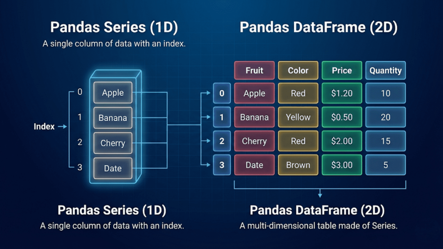
A Pandas Series is a one-dimensional labeled array capable of holding any data type, while a Pandas DataFrame is a two-dimensional table of data with labeled rows and columns — think of a Series as a single spreadsheet column and a DataFrame as the entire spreadsheet. Together, these two Pandas data structures form the foundation of nearly all data manipulation in Python.
Introduction: Why Pandas Series and DataFrame Matter
When you first encounter Pandas in a data science course or tutorial, you will immediately come across two objects that appear constantly: the Series and the DataFrame. Both are central to the Pandas library, and both are used in virtually every data science workflow. Yet many beginners treat them interchangeably or feel confused about when to use one versus the other.
Understanding the distinction between a Pandas Series and a Pandas DataFrame is not merely a matter of academic curiosity — it is a practical skill that will help you write cleaner, more efficient code, debug problems faster, and understand what Pandas functions actually return. In this article, you will gain a thorough understanding of both data structures, learn how to create and manipulate them, and discover through practical examples exactly where each one fits in real data science workflows.
Pandas data structures were designed by Wes McKinney while he was working at AQR Capital Management, and the library was first released publicly in 2008. The name “Pandas” is derived from the econometrics term “Panel Data” — multi-dimensional structured data sets. From the very beginning, the library was designed around two primary abstractions: the one-dimensional Series and the two-dimensional DataFrame. Understanding both is essential to mastering Pandas.
1. What Is a Pandas Series?
A Pandas Series is a one-dimensional array-like object that can hold data of any type — integers, floats, strings, booleans, Python objects, and more. What sets a Series apart from a plain Python list or a NumPy array is that every element in a Series has a label, called an index. This index allows you to access elements by label rather than just by position.
Think of a Series as a single column in a spreadsheet. The column has a name, each row has a label (row number or custom label), and all the values in the column share the same data type. This is exactly how a Pandas Series works.
1.1 Creating a Pandas Series
You can create a Series in several ways. The most common approach is to pass a Python list or a NumPy array to pd.Series():
import pandas as pd
import numpy as np

# Creating a Series from a list
temperatures = pd.Series([23.5, 25.1, 19.8, 27.4, 22.0])
print(temperatures)

# Output:
# 0    23.5
# 1    25.1
# 2    19.8
# 3    27.4
# 4    22.0
# dtype: float64Notice that Pandas automatically assigned integer labels (0, 1, 2, 3, 4) as the index. These are the default labels when you do not specify an index. The dtype at the bottom tells you the data type of the values in the Series — in this case, 64-bit floating point numbers.
You can also supply custom index labels, which is one of the most powerful features of a Series:
# Creating a Series with custom index labels
city_temps = pd.Series(
    [23.5, 25.1, 19.8, 27.4, 22.0],
    index=['New York', 'Los Angeles', 'Chicago', 'Houston', 'Phoenix']
)
print(city_temps)

# Output:
# New York       23.5
# Los Angeles    25.1
# Chicago        19.8
# Houston        27.4
# Phoenix        22.0
# dtype: float64Now each temperature value is associated with a city name. You can access data by label: city_temps['Chicago'] returns 19.8, and city_temps['Houston'] returns 27.4. This is far more readable and practical than using raw integer positions.
You can also create a Series from a Python dictionary, where the dictionary keys become the index:
# Creating a Series from a dictionary
sales_data = {'Jan': 15000, 'Feb': 18500, 'Mar': 21000, 'Apr': 17300}
monthly_sales = pd.Series(sales_data)
print(monthly_sales)

# Output:
# Jan    15000
# Feb    18500
# Mar    21000
# Apr    17300
# dtype: int641.2 Key Attributes of a Pandas Series
Every Pandas Series has several important attributes that tell you about its structure and contents:
s = pd.Series([10, 20, 30, 40, 50], index=['a', 'b', 'c', 'd', 'e'])

print(s.values)    # array([10, 20, 30, 40, 50]) — underlying NumPy array
print(s.index)     # Index(['a','b','c','d','e'], dtype='object')
print(s.dtype)     # int64
print(s.shape)     # (5,) — a tuple with one dimension
print(s.name)      # None — unless you assign a name
print(len(s)) # 5The name attribute of a Series is particularly important when a Series becomes a column in a DataFrame — the Series name becomes the column label. This connection between Series and DataFrame is a concept you will explore more deeply as you continue through this guide.
1.3 Accessing Elements in a Series
Pandas provides two primary ways to access elements in a Series: label-based access with .loc and position-based access with .iloc. Understanding the difference between these two is crucial for avoiding subtle bugs in your code.
city_temps = pd.Series(
    [23.5, 25.1, 19.8, 27.4],
    index=['New York', 'Los Angeles', 'Chicago', 'Houston']
)

# Label-based access
print(city_temps.loc['Chicago'])    # 19.8

# Position-based access
print(city_temps.iloc[2])           # 19.8 (Chicago is at position 2)

# Slicing with loc (inclusive of both endpoints)
print(city_temps.loc['New York':'Chicago'])

# Slicing with iloc (exclusive of end position)
print(city_temps.iloc[0:2])Pro Tip: When your index consists of integers, using
[]directly can be ambiguous — Pandas may interpret it as either a label or a position. Always use.loc[]for label-based access and.iloc[]for position-based access to write unambiguous code.
1.4 Vectorized Operations on a Series
One of the most powerful features of a Pandas Series is that it supports vectorized operations — mathematical operations are applied to every element simultaneously, without writing a loop. This is inherited from NumPy and makes your code both faster and more readable.
prices = pd.Series([100, 200, 150, 300, 250])

# Apply a 10% discount to every price
discounted = prices * 0.90
print(discounted)
# 0     90.0
# 1    180.0
# 2    135.0
# 3    270.0
# 4    225.0

# Apply a function to every element
log_prices = np.log(prices)
print(log_prices)You can also perform arithmetic between two Series. Pandas will automatically align the operations based on the index labels — a uniquely powerful feature called index alignment. This means that if two Series share some index labels but not all, Pandas aligns them correctly and introduces NaN (Not a Number) for labels present in one Series but not the other.
s1 = pd.Series([10, 20, 30], index=['a', 'b', 'c'])
s2 = pd.Series([5, 10, 15], index=['b', 'c', 'd'])

result = s1 + s2
print(result)
# a     NaN   (a is in s1 but not s2)
# b    25.0   (s1['b']=20, s2['b']=5 => 25)
# c    40.0   (s1['c']=30, s2['c']=10 => 40)
# d NaN (d is in s2 but not s1)This index alignment behavior is one of the most distinctive and useful aspects of Pandas. It means you rarely have to manually worry about matching up rows — Pandas handles it for you based on the index labels.
2. What Is a Pandas DataFrame?
A Pandas DataFrame is a two-dimensional, size-mutable, tabular data structure with labeled rows and columns. Think of it as a spreadsheet, a SQL table, or a dictionary of Pandas Series objects that all share the same index. The DataFrame is the workhorse of data science in Python — nearly every dataset you will ever work with gets loaded into a DataFrame.
Conceptually, a DataFrame consists of multiple Series, each representing a column, all sharing the same row index. Every column in a DataFrame can have its own data type (dtype), so you can have a mix of integers, floats, strings, and booleans — each in its own column — within a single DataFrame.
2.1 Creating a Pandas DataFrame
The most common way to create a DataFrame is from a dictionary of lists, where each key becomes a column name:
import pandas as pd

# Creating a DataFrame from a dictionary
data = {
    'Name':       ['Alice', 'Bob', 'Charlie', 'Diana', 'Edward'],
    'Age':        [28, 34, 25, 31, 40],
    'Department': ['Engineering', 'Marketing', 'Engineering', 'HR', 'Finance'],
    'Salary':     [85000, 72000, 78000, 65000, 95000],
    'Remote':     [True, False, True, True, False]
}

employees = pd.DataFrame(data)
print(employees)

#       Name  Age   Department  Salary  Remote
# 0    Alice   28  Engineering   85000    True
# 1      Bob   34    Marketing   72000   False
# 2  Charlie   25  Engineering   78000    True
# 3    Diana   31           HR   65000    True
# 4 Edward 40 Finance 95000 FalseYou can also create a DataFrame from a list of dictionaries (where each dictionary represents one row), from a NumPy array, from a CSV file using pd.read_csv(), or from another DataFrame. In practice, the most common way to get a DataFrame is by reading data from an external source such as a CSV file or a database.
# Creating from a list of dictionaries (each dict = one row)
records = [
    {'product': 'Laptop',  'price': 999.99, 'units': 150},
    {'product': 'Mouse',   'price': 29.99,  'units': 500},
    {'product': 'Monitor', 'price': 349.99, 'units': 200},
]
products_df = pd.DataFrame(records)

# Creating from a NumPy array
import numpy as np
matrix = np.array([[1, 2, 3], [4, 5, 6], [7, 8, 9]])
df_from_array = pd.DataFrame(matrix, columns=['A', 'B', 'C'])2.2 Key Attributes of a Pandas DataFrame
Like a Series, a DataFrame has several essential attributes that help you understand its structure at a glance:
df = pd.DataFrame({
    'A': [1, 2, 3],
    'B': [4.0, 5.0, 6.0],
    'C': ['x', 'y', 'z']
})

print(df.shape)        # (3, 3) — 3 rows, 3 columns
print(df.columns)      # Index(['A', 'B', 'C'], dtype='object')
print(df.index)        # RangeIndex(start=0, stop=3, step=1)
print(df.dtypes)       # A: int64, B: float64, C: object
print(df.values)       # 2D NumPy array of all values
print(df.info())       # Summary: shape, dtypes, memory usage
print(df.describe()) # Statistical summary of numeric columnsThe df.info() method is particularly useful when you first load a dataset — it shows you every column name, how many non-null values each column has, and the data type of each column. The df.describe() method gives you statistical summaries (mean, standard deviation, min, max, and quartiles) for all numeric columns in one glance.
2.3 Selecting Data from a DataFrame
Selecting data from a DataFrame is slightly more complex than selecting from a Series, because you now have both rows and columns to navigate. The primary methods are column selection, .loc[], .iloc[], and boolean indexing.
employees = pd.DataFrame({
    'Name':   ['Alice', 'Bob', 'Charlie', 'Diana', 'Edward'],
    'Age':    [28, 34, 25, 31, 40],
    'Salary': [85000, 72000, 78000, 65000, 95000]
})

# --- Selecting columns ---
# Single column → returns a Series
name_series = employees['Name']
print(type(name_series))   # <class 'pandas.core.series.Series'>

# Multiple columns → returns a DataFrame
subset_df = employees[['Name', 'Salary']]
print(type(subset_df))     # <class 'pandas.core.frame.DataFrame'>

# --- Selecting rows and columns with .loc ---
print(employees.loc[1:3])                        # Rows 1 to 3, all columns
print(employees.loc[0:2, ['Name', 'Age']])       # Specific rows and columns

# --- Selecting by position with .iloc ---
print(employees.iloc[0, 0])       # 'Alice' (row 0, column 0)
print(employees.iloc[1:3, 1:])   # rows 1-2, columns 1 onwards

# --- Boolean indexing (filtering) ---
high_earners = employees[employees['Salary'] > 75000]
print(high_earners)Key Insight: Selecting a single column from a DataFrame with single brackets
df['ColumnName']returns a Series. Selecting one or more columns with double bracketsdf[['Col1', 'Col2']]returns a DataFrame. This is a common source of confusion for beginners.
3. Pandas Series vs DataFrame: A Complete Comparison
Now that you understand both structures individually, let us compare them directly. The table below summarizes the most important differences between a Pandas Series and a Pandas DataFrame.
| Feature | Pandas Series | Pandas DataFrame |
|---|---|---|
| Dimensions | 1-Dimensional (1D) | 2-Dimensional (2D) |
| Structure | Single column of data with index | Rows and columns (like a table) |
| Data Types | Homogeneous (one dtype) | Heterogeneous (mixed dtypes allowed) |
| Index | Single index (row labels) | Row index + column labels |
| Creation | pd.Series([1, 2, 3]) | pd.DataFrame({...}) |
| Shape | Returns (n,) — a single number | Returns (rows, cols) — a tuple |
| Access | series[label] or series[0] | df['col'] or df.loc[row, col] |
| SQL Equivalent | Single column result set | Full table / query result |
| Common Use | Single feature or target variable | Full dataset with multiple features |
| Memory | Less overhead (simpler structure) | More overhead (manages 2D metadata) |
| Iteration | Iterates over values | Iterates over column names by default |
| Arithmetic | Element-wise on values | Element-wise aligned on index & columns |
The most important practical takeaway is that a Series represents a single variable or feature, while a DataFrame represents an entire dataset with multiple variables. In machine learning workflows, for example, you will often have a DataFrame X containing all your features (predictors) and a Series y containing your target variable (the outcome you want to predict).
4. The Deep Relationship Between Series and DataFrame
One of the most important concepts to understand is that a DataFrame is fundamentally a container for Series objects. When you access a single column from a DataFrame, you get a Series back. When you create a DataFrame from a dictionary, each value in the dictionary is typically a list that becomes a Series. When you perform operations column by column in a DataFrame, you are typically working with Series objects under the hood.
4.1 A DataFrame Is a Collection of Series
You can think of a DataFrame as a dictionary of Series objects, where all the Series share the same index. Here is a direct demonstration:
import pandas as pd

# Build a DataFrame from individual Series
name_series   = pd.Series(['Alice', 'Bob', 'Charlie'], name='Name')
age_series    = pd.Series([28, 34, 25], name='Age')
salary_series = pd.Series([85000, 72000, 78000], name='Salary')

# Combine Series into a DataFrame
df = pd.concat([name_series, age_series, salary_series], axis=1)
print(df)

#       Name  Age  Salary
# 0    Alice   28   85000
# 1      Bob   34   72000
# 2 Charlie 25 78000The axis=1 argument in pd.concat() tells Pandas to concatenate the Series side by side (along the column axis) rather than stacking them vertically. Each Series becomes one column in the resulting DataFrame.
You can also verify this relationship by extracting a column from a DataFrame:
# Extract a column from DataFrame → get a Series
salary_col = df['Salary']
print(type(salary_col))   # <class 'pandas.core.series.Series'>
print(salary_col.name)    # 'Salary'

# Verify: the Series index matches the DataFrame index
print(salary_col.index) # RangeIndex(start=0, stop=3, step=1)4.2 Index Alignment Across Operations
The shared index between a Series and a DataFrame is not just cosmetic — it enables powerful alignment behavior when you perform operations. When you add a Series to a DataFrame or use a Series to filter rows of a DataFrame, Pandas automatically aligns the data by index.
df = pd.DataFrame({
    'Price':    [100, 200, 150, 300],
    'Quantity': [10, 5, 8, 3]
})

# Create a new column by multiplying two existing columns
# Each column is a Series; the result is also a Series
df['Revenue'] = df['Price'] * df['Quantity']
print(df)

#    Price  Quantity  Revenue
# 0    100        10     1000
# 1    200         5     1000
# 2    150         8     1200
# 3 300 3 900When you multiply two columns of a DataFrame, you are actually multiplying two Series. The result is a new Series, which you can immediately add back to the DataFrame as a new column. This is one of the most fundamental patterns in Pandas data manipulation.
5. Real-World Use Cases: When to Use Series vs DataFrame
Understanding the theoretical difference between Series and DataFrame is important, but knowing when to use each in practice is what makes you an effective data scientist. Here are the most common real-world scenarios.
5.1 Feature Engineering: Working Between Series and DataFrame
Feature engineering is the process of creating new variables from existing ones in your dataset. This workflow constantly moves between Series and DataFrame operations:
import pandas as pd
import numpy as np

# Sample e-commerce dataset
orders = pd.DataFrame({
    'order_id':        [1001, 1002, 1003, 1004, 1005],
    'purchase_amount': [250.00, 89.99, 499.50, 35.00, 120.75],
    'discount_pct':    [0.10, 0.05, 0.20, 0.00, 0.15],
    'customer_id':     [201, 202, 201, 203, 202]
})

# Feature 1: Final price after discount (Series operation → new column)
orders['final_price'] = orders['purchase_amount'] * (1 - orders['discount_pct'])

# Feature 2: Is this a premium order? (Boolean Series)
orders['is_premium'] = orders['final_price'] > 200

# Feature 3: Log-transform the price (Series → Series)
orders['log_price'] = np.log1p(orders['final_price'])

print(orders.head())In this example, every new column you create is generated by performing operations on Series (the columns of the DataFrame). The result of each operation is a new Series, which you assign back to the DataFrame with a new column name. This pattern — extract Series, transform it, assign it back — is central to data science workflows.
5.2 Machine Learning: Series as Target Variable
In supervised machine learning, you typically split your data into features (X) and a target variable (y). The features are stored in a DataFrame, and the target is stored in a Series:
from sklearn.linear_model import LinearRegression

# X is a DataFrame containing the feature columns
X = orders[['purchase_amount', 'discount_pct', 'log_price']]

# y is a Series containing the target
y = orders['final_price']

print(f'X type: {type(X)}')   # DataFrame
print(f'X shape: {X.shape}')  # (5, 3)
print(f'y type: {type(y)}')   # Series
print(f'y shape: {y.shape}')  # (5,)

# Scikit-learn accepts both DataFrame X and Series y
model = LinearRegression()
model.fit(X, y)This is the standard pattern used across virtually every machine learning workflow. Understanding that X is a DataFrame and y is a Series helps you immediately grasp the shape of your data problem.
5.3 Time Series Analysis: Series at Its Best
When working with time series data — stock prices, weather readings, sales over time — a Pandas Series with a DatetimeIndex is often the ideal data structure:
import pandas as pd

# Daily stock prices (simplified)
dates = pd.date_range(start='2024-01-01', periods=10, freq='B')  # business days
prices = pd.Series(
    [150.20, 152.40, 149.80, 153.60, 151.90,
     155.10, 157.20, 154.80, 158.30, 160.00],
    index=dates,
    name='AAPL'
)

# Calculate 3-day rolling average (moving average)
rolling_avg = prices.rolling(window=3).mean()

# Calculate daily returns
daily_returns = prices.pct_change()

print(prices.head())
print(f'\nMean price: {prices.mean():.2f}')
print(f'Max price:  {prices.max():.2f}')
print(f'Volatility: {daily_returns.std():.4f}')A Pandas Series with a DatetimeIndex unlocks powerful time-series-specific methods like rolling(), shift(), resample(), and diff() — all of which operate element-wise along the time axis. For time series with a single variable (one stock, one sensor reading, one temperature measurement), a Series is the natural choice.
When you have multiple time series that you want to analyze together — for example, prices of multiple stocks — that is when you move to a DataFrame, with one column per stock and a shared DatetimeIndex as the row index.
5.4 Groupby and Aggregation: Working with Both
The groupby operation is one of the most powerful patterns in Pandas, and it naturally bridges Series and DataFrame:
employees = pd.DataFrame({
    'Name':       ['Alice', 'Bob', 'Charlie', 'Diana', 'Edward', 'Fiona'],
    'Department': ['Eng', 'Mkt', 'Eng', 'HR', 'Finance', 'Mkt'],
    'Salary':     [85000, 72000, 78000, 65000, 95000, 68000],
    'Years_Exp':  [4, 7, 3, 8, 12, 2]
})

# Group by Department and compute mean of all numeric columns → DataFrame
dept_stats = employees.groupby('Department').mean(numeric_only=True)
print(type(dept_stats))   # DataFrame
print(dept_stats)

# Group by Department and compute mean of a SINGLE column → Series
avg_salary = employees.groupby('Department')['Salary'].mean()
print(type(avg_salary))   # Series
print(avg_salary)When you apply aggregation to all numeric columns in a grouped DataFrame, you get a DataFrame back. When you apply aggregation to a single column (which is a Series), you get a Series back. This consistent behavior makes it easy to predict what type of result you will get.
6. Common Operations and Conversions Between Series and DataFrame
In real data science work, you will constantly convert between Series and DataFrame. Knowing the most common conversion patterns will save you significant time and prevent confusion.
6.1 Converting a Series to a DataFrame
s = pd.Series([10, 20, 30, 40], name='values')

# Method 1: Use .to_frame()
df = s.to_frame()
print(df)
#    values
# 0      10
# 1      20
# 2      30
# 3      40

# Method 2: Override the column name
df_renamed = s.to_frame(name='new_column_name')

# Method 3: Use pd.DataFrame constructor
df2 = pd.DataFrame({'values': s})The .to_frame() method is the cleanest way to convert a Series to a one-column DataFrame. This is useful when a function requires a DataFrame input but you only have a Series, or when you want to join a Series to an existing DataFrame using a merge operation.
6.2 Converting a DataFrame to a Series
df = pd.DataFrame({
    'A': [1, 2, 3],
    'B': [4, 5, 6]
})

# Method 1: Select a single column
series_a = df['A']   # Returns a Series

# Method 2: Use .squeeze() on a single-column DataFrame
single_col_df = df[['A']]          # Still a DataFrame
series_squeezed = single_col_df.squeeze()  # Converts to Series

# Method 3: Stack a DataFrame to a Series (multi-level index)
stacked = df.stack()  # Converts 2D DataFrame to 1D Series with MultiIndex
print(stacked)6.3 Checking the Type of Your Object
A very common source of bugs in Pandas code is not knowing whether you have a Series or a DataFrame at a given point in your code. Use isinstance() or type() to check:
import pandas as pd

def check_pandas_type(obj):
    if isinstance(obj, pd.DataFrame):
        print(f'DataFrame with shape {obj.shape}')
    elif isinstance(obj, pd.Series):
        print(f'Series with {len(obj)} elements, dtype={obj.dtype}')
    else:
        print(f'Unknown type: {type(obj)}')

df = pd.DataFrame({'x': [1, 2, 3], 'y': [4, 5, 6]})
check_pandas_type(df)          # DataFrame with shape (3, 2)
check_pandas_type(df['x'])    # Series with 3 elements, dtype=int64
check_pandas_type(df[['x']]) # DataFrame with shape (3, 1)7. Performance Considerations
For most everyday data science tasks — datasets with thousands to low millions of rows — the performance difference between Series and DataFrame operations is negligible. However, understanding the underlying performance characteristics can help you write more efficient code.
Both Pandas Series and DataFrame are built on top of NumPy arrays under the hood, which means their numeric operations are highly optimized and run at native C speed. The key performance principles to keep in mind are:
- Avoid Python loops: Always prefer vectorized operations over iterating through rows with
forloops or.iterrows(). Vectorized operations on Series and DataFrame columns are orders of magnitude faster. - Use appropriate dtypes: A Series of integers uses far less memory than a Series of Python objects. Use
pd.to_numeric(),pd.to_datetime(), and.astype()to ensure your data has the most efficient dtype. - Minimize copying: Operations like filtering create new objects. When working with very large datasets, be mindful of how many intermediate copies you create.
- Use
.valuesfor pure NumPy speed: If you need maximum performance for a numerical computation, extract the underlying NumPy array with.valuesand perform the operation directly on the array.
import pandas as pd
import time

large_series = pd.Series(range(1_000_000))

# Slow approach: Python loop
start = time.time()
result_loop = []
for val in large_series:
    result_loop.append(val * 2)
print(f'Loop time: {time.time()-start:.3f}s')       # ~0.5 seconds

# Fast approach: vectorized operation
start = time.time()
result_vec = large_series * 2
print(f'Vectorized time: {time.time()-start:.3f}s') # ~0.005 secondsThe vectorized approach is typically 100x faster than the equivalent Python loop. This difference becomes critically important when working with datasets of millions of rows, which are common in real-world data science projects.
8. Common Pitfalls and How to Avoid Them
Even experienced data scientists occasionally fall into these traps when working with Pandas Series and DataFrames. Being aware of them will save you significant debugging time.
8.1 The SettingWithCopyWarning
One of the most common warnings you will encounter is SettingWithCopyWarning. It occurs when you try to modify a slice of a DataFrame, which may or may not modify the original DataFrame depending on how Pandas decides to handle it internally:
df = pd.DataFrame({'A': [1, 2, 3, 4, 5], 'B': [10, 20, 30, 40, 50]})

# PROBLEMATIC: chained indexing (may not modify original df)
df[df['A'] > 2]['B'] = 999   # SettingWithCopyWarning!

# CORRECT: use .loc for safe in-place modification
df.loc[df['A'] > 2, 'B'] = 999
print(df)Always use .loc[] or .iloc[] for assignments that modify the DataFrame. Avoid chained indexing (applying two sets of brackets in sequence) for assignment operations.
8.2 Confusing Single vs Double Brackets for Column Selection
As mentioned earlier, the number of brackets you use when selecting columns determines whether you get a Series or a DataFrame:
df = pd.DataFrame({'A': [1, 2, 3], 'B': [4, 5, 6], 'C': [7, 8, 9]})

col_series = df['A']       # Series — single column
col_df     = df[['A']]     # DataFrame — single column as 1-col DataFrame
multi_df   = df[['A','B']] # DataFrame — two columns

print(type(col_series))    # pandas.core.series.Series
print(type(col_df)) # pandas.core.frame.DataFrameThis distinction matters when calling functions that specifically require a DataFrame or a Series. For example, many scikit-learn transformers require a DataFrame input, not a Series.
8.3 Index Misalignment During Filtering
When you filter a DataFrame or Series, the original index values are preserved — they are not reset. This can cause unexpected behavior when you subsequently try to use the filtered object:
df = pd.DataFrame({'A': [10, 20, 30, 40, 50]})

# Filter: keep only rows where A > 20
filtered = df[df['A'] > 20]
print(filtered)
# Index is 2, 3, 4 (not 0, 1, 2!)
#    A
# 2  30
# 3  40
# 4  50

# If you need sequential index, reset it:
filtered_reset = filtered.reset_index(drop=True)
print(filtered_reset)
#    A
# 0  30
# 1  40
# 2 50The reset_index(drop=True) call resets the index to a clean sequential range starting from 0. The drop=True argument prevents the old index from being added as a new column (which is the default behavior of reset_index).
8.4 Forgetting That String Operations Require .str
When you have a Series of strings (dtype='object'), standard Python string methods do not work directly. You must use the .str accessor:
names = pd.Series(['alice smith', 'bob jones', 'charlie brown'])

# WRONG — this does not apply .upper() to each element
# names.upper()   # AttributeError

# CORRECT — use the .str accessor
print(names.str.upper())
# 0    ALICE SMITH
# 1      BOB JONES
# 2  CHARLIE BROWN

# Extract first name
first_names = names.str.split().str[0]
print(first_names)
# 0      alice
# 1        bob
# 2 charlie9. Advanced Topics: MultiIndex and Beyond
Once you are comfortable with basic Series and DataFrame operations, you can explore more advanced indexing concepts that give Pandas additional expressive power for complex, hierarchical data.
9.1 MultiIndex Series
A MultiIndex (or hierarchical index) allows a Series or DataFrame to have multiple levels of row labels. This is useful for representing data that has a natural hierarchy, such as sales data grouped by year and quarter, or population data grouped by country and city.
import pandas as pd

# Create a MultiIndex Series
index = pd.MultiIndex.from_tuples([
    ('2023', 'Q1'), ('2023', 'Q2'), ('2023', 'Q3'), ('2023', 'Q4'),
    ('2024', 'Q1'), ('2024', 'Q2'), ('2024', 'Q3'), ('2024', 'Q4'),
], names=['Year', 'Quarter'])

revenue = pd.Series(
    [125000, 138000, 142000, 165000, 148000, 162000, 155000, 189000],
    index=index,
    name='Revenue'
)

print(revenue)
print('\n2023 Revenue:')
print(revenue['2023'])           # Select all 2023 data
print(revenue['2024', 'Q3']) # Select specific period9.2 Wide vs Long Format DataFrames
An important concept in data reshaping is the difference between wide-format and long-format DataFrames. Understanding this — and when to convert between the two — is essential for data visualization with libraries like Seaborn or for certain statistical analyses.
# Wide format: each variable is a column
wide_df = pd.DataFrame({
    'Student': ['Alice', 'Bob', 'Charlie'],
    'Math':    [90, 75, 88],
    'Science': [85, 92, 79],
    'English': [78, 83, 95]
})

# Convert to long format using pd.melt()
long_df = pd.melt(
    wide_df,
    id_vars=['Student'],
    value_vars=['Math', 'Science', 'English'],
    var_name='Subject',
    value_name='Score'
)
print(long_df)
#     Student  Subject  Score
# 0     Alice     Math     90
# 1       Bob     Math     75
# 2   Charlie     Math     88
# 3     Alice  Science     85
# ... and so onIn long format, there is one row per observation per variable. In wide format, there is one row per subject with separate columns for each variable. Long format is required by many visualization libraries and statistical models. Wide format is often more natural for human-readable reporting. Pandas provides pd.melt() to go from wide to long, and df.pivot() or df.pivot_table() to go from long to wide.
10. Putting It All Together: A Mini Data Analysis Project
Let us apply everything you have learned in a complete mini-project that moves through data loading, exploration, feature engineering, and analysis — while demonstrating natural transitions between Series and DataFrame.
import pandas as pd
import numpy as np

# Simulate a retail sales dataset
np.random.seed(42)
n = 1000

df = pd.DataFrame({
    'date':        pd.date_range('2024-01-01', periods=n, freq='h'),
    'product_id':  np.random.choice(['A', 'B', 'C', 'D'], n),
    'units_sold':  np.random.randint(1, 50, n),
    'unit_price':  np.random.choice([9.99, 19.99, 49.99, 99.99], n),
    'region':      np.random.choice(['North', 'South', 'East', 'West'], n)
})

# Step 1: Explore the DataFrame
print(df.shape)         # (1000, 5)
print(df.dtypes)
print(df.describe())

# Step 2: Feature engineering — Series operations on DataFrame columns
df['revenue']  = df['units_sold'] * df['unit_price']
df['month']    = df['date'].dt.month
df['hour']     = df['date'].dt.hour
df['weekday']  = df['date'].dt.day_name()

# Step 3: Aggregate by product — single column → Series
product_revenue = df.groupby('product_id')['revenue'].sum()
print(type(product_revenue))  # Series
print(product_revenue.sort_values(ascending=False))

# Step 4: Aggregate multiple metrics → DataFrame
product_stats = df.groupby('product_id').agg(
    total_revenue=('revenue', 'sum'),
    avg_units=('units_sold', 'mean'),
    num_transactions=('units_sold', 'count')
)
print(type(product_stats))  # DataFrame
print(product_stats)

# Step 5: Find the best region → scalar from Series
best_region = df.groupby('region')['revenue'].sum().idxmax()
print(f'Best performing region: {best_region}')This mini-project demonstrates the natural rhythm of real data science work: you start with a DataFrame, perform Series operations to engineer new features, then aggregate and analyze using both Series (for single metrics) and DataFrames (for multiple metrics). The transition between the two structures happens fluidly and naturally.
11. Best Practices for Working with Series and DataFrame
After years of community experience with Pandas, several best practices have emerged that will help you write cleaner, more maintainable, and more efficient data science code.
- Know what you are working with: At every step of your analysis, be aware of whether you have a Series or a DataFrame. Use
print(type(obj))orprint(obj.shape)liberally when debugging. - Use method chaining: Pandas supports method chaining, which lets you apply multiple transformations in sequence without creating many intermediate variables, making your code more readable.
- Avoid modifying views: Use
.copy()when you want to create an independent copy of a DataFrame slice to avoidSettingWithCopyWarningand potential data corruption. - Name your Series: When creating a standalone Series, always give it a meaningful
nameattribute (pd.Series([...], name='column_name')). This name becomes the column label when the Series is added to a DataFrame. - Prefer
.locand.iloc: Always use explicit label-based (.loc) or position-based (.iloc) indexing for assignment operations. Never chain indexers for assignments. - Reset the index after filtering: If you filter a DataFrame and then want a clean sequential index, use
reset_index(drop=True)to avoid index gaps and potential alignment issues downstream. - Validate your data types: After loading data or performing merges, always call
df.dtypesanddf.info()to verify that column types are what you expect. Numeric columns loaded as strings are a common source of subtle bugs.
Conclusion: Mastering the Core Pandas Data Structures
Understanding the difference between a Pandas Series and a Pandas DataFrame is foundational to becoming an effective data scientist. The Series is your one-dimensional workhorse for single variables, time series, and intermediate calculations. The DataFrame is your two-dimensional canvas for complete datasets with multiple features.
The two structures are deeply intertwined: every DataFrame column is a Series, and multiple aligned Series together form a DataFrame. Operations on a DataFrame often produce Series (when you select a single column or aggregate along one axis), and Series can be assembled into DataFrames (using pd.concat or pd.DataFrame). Mastering this relationship — knowing what type of object your code is producing at each step — will make you a far more confident and capable data scientist.
As you continue your data science journey, you will encounter these structures constantly. Whether you are building machine learning models in scikit-learn, creating visualizations with Matplotlib or Seaborn, or performing time series analysis, your starting point will almost always be a Pandas Series or DataFrame. The effort you invest now in understanding these two structures will pay dividends throughout your entire career.
In the next article, we will cover handling missing data in Pandas — a critical skill that builds directly on what you have learned here about Series and DataFrame operations.
Key Takeaways
- A Pandas Series is a one-dimensional labeled array; a Pandas DataFrame is a two-dimensional table with labeled rows and columns.
- A DataFrame can be understood as a collection of Series objects that share the same row index.
- Selecting a single column from a DataFrame with
df['col']returns a Series; selecting withdf[['col']]returns a single-column DataFrame. - Both Series and DataFrame support vectorized operations inherited from NumPy, making computation fast and code concise.
- Index alignment is a powerful feature of Pandas — arithmetic operations between two Series or between Series and DataFrames automatically align by index label.
- In machine learning, features (X) are typically stored as a DataFrame while the target variable (y) is stored as a Series.
- Always use
.loc[]for label-based indexing and.iloc[]for position-based indexing to write unambiguous, bug-free code. - Use
isinstance(obj, pd.Series)orisinstance(obj, pd.DataFrame)to check the type of your Pandas objects when debugging.