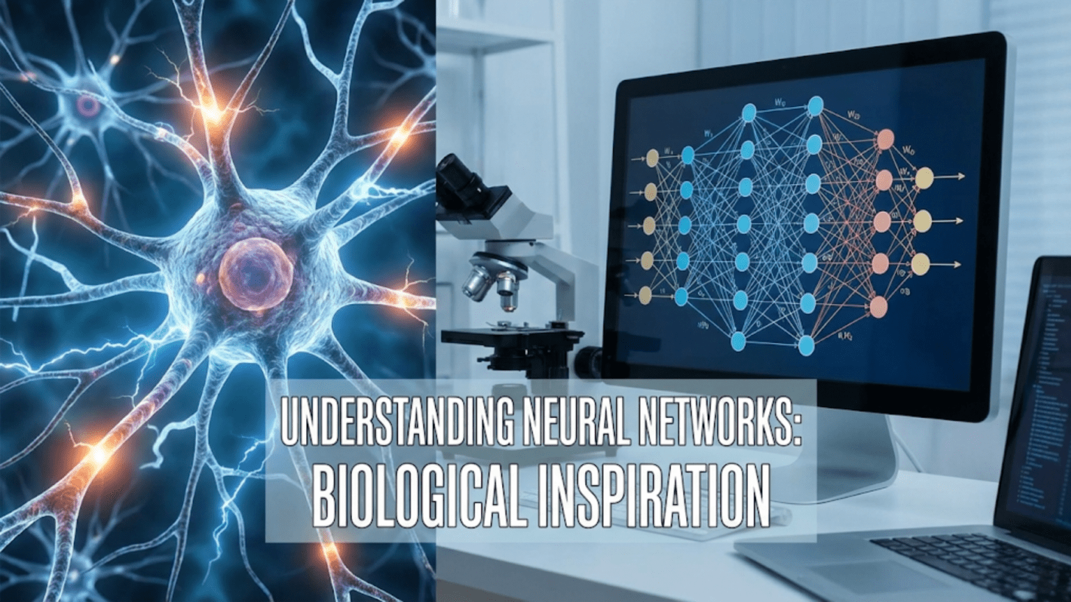
Artificial neural networks are computational models inspired by biological neural networks in the brain. Like biological neurons that receive signals through dendrites, process them in the cell body, and transmit outputs via axons, artificial neurons receive weighted inputs, apply activation functions, and produce outputs. Networks connect multiple artificial neurons in layers, mimicking how billions of interconnected biological neurons in the brain learn patterns through strengthening and weakening connections based on experience.
Introduction: Learning from Nature’s Most Powerful Computer
The human brain is the most sophisticated information processing system known to exist. With roughly 86 billion neurons connected through trillions of synapses, it performs feats that still surpass our most advanced computers: recognizing faces instantaneously, understanding language naturally, learning new skills from limited examples, and adapting to changing environments seamlessly.
What if we could build machines that learn the same way brains do? This question has driven one of the most successful ideas in artificial intelligence: neural networks. These computational models draw inspiration from biological neural networks, attempting to replicate—in simplified form—the mechanisms that allow brains to learn and process information.
The connection between biological and artificial neural networks isn’t just historical curiosity—understanding the biological inspiration provides crucial insights into why neural networks work, their capabilities and limitations, and how to design better architectures. The brain’s parallel processing, distributed representations, and ability to learn from experience directly influenced the design principles of modern deep learning.
Yet it’s important to understand both the inspiration and the reality: artificial neural networks are inspired by biology but are ultimately simplified mathematical models. They capture some brain-like properties while diverging significantly in others. Understanding what aspects are biologically inspired and which are engineering choices helps develop accurate intuitions about how these powerful systems work.
This comprehensive guide explores the biological foundations of artificial neural networks. You’ll learn how biological neurons work, how brains process information, how these biological concepts translated to artificial systems, where the parallels hold and where they break down, and what modern neuroscience continues to teach us about building intelligent machines.
The Biological Neuron: Nature’s Computing Unit
To understand artificial neural networks, we must first understand their biological inspiration: the neuron.
Anatomy of a Biological Neuron
A neuron is a specialized cell designed to receive, process, and transmit information through electrical and chemical signals.
Key Components:
1. Dendrites:
- Branch-like structures extending from cell body
- Function: Receive signals from other neurons
- Multiple dendrites per neuron (hundreds to thousands)
- Act as input channels
2. Cell Body (Soma):
- Contains the nucleus and cell machinery
- Function: Integrates incoming signals
- Sums up excitatory and inhibitory inputs
- Determines whether to fire
3. Axon:
- Long fiber extending from cell body
- Function: Transmits output signal
- Can be very long (up to 1 meter in humans)
- Single axon per neuron
4. Axon Terminals (Synaptic Terminals):
- Branches at axon end
- Function: Connect to other neurons
- Release neurotransmitters
- Each terminal forms a synapse
5. Synapses:
- Junction between neurons
- Function: Transmit signals between neurons
- Chemical transmission via neurotransmitters
- Plastic—strengthen or weaken with use
How Biological Neurons Communicate
The Process:
Step 1: Receiving Signals (Dendrites)
- Other neurons send signals to dendrites
- Each synapse can be excitatory (+) or inhibitory (-)
- Signals flow into cell body
Step 2: Integration (Cell Body)
- Cell body sums all incoming signals
- Weighted sum: stronger synapses contribute more
- Temporal summation: signals arriving close in time add up
Step 3: Activation Decision
- If total signal exceeds threshold: neuron “fires”
- Generates action potential (electrical spike)
- All-or-nothing response
- If below threshold: no firing
Step 4: Signal Transmission (Axon)
- Action potential travels down axon
- Speed: 1-100 meters per second
- Signal doesn’t weaken over distance
Step 5: Synaptic Transmission
- Electrical signal reaches axon terminals
- Triggers neurotransmitter release
- Neurotransmitters cross synaptic gap
- Activate receptors on next neuron’s dendrites
Step 6: Synaptic Plasticity
- Frequently used synapses strengthen
- Rarely used synapses weaken
- “Neurons that fire together, wire together” (Hebb’s rule)
- This is how learning occurs biologically
Key Properties
1. Threshold Activation:
- Neurons don’t gradually respond
- All-or-nothing firing
- Threshold determines firing
2. Weighted Inputs:
- Different synapses have different strengths
- Strong synapses contribute more to activation
- Synaptic weights encode learned information
3. Parallel Processing:
- Billions of neurons operate simultaneously
- Massive parallelism enables fast processing
4. Plasticity:
- Connections change with experience
- Learning modifies synaptic strengths
- Brain rewires itself continuously
5. Distributed Representation:
- Information stored across many neurons
- No single neuron stores a concept
- Patterns of activity represent information
From Biology to Mathematics: The Artificial Neuron
Scientists abstracted biological neurons into mathematical models, creating artificial neurons.
The Mathematical Model
An artificial neuron (also called perceptron or node) is a simplified mathematical representation:
Structure:
Inputs (x₁, x₂, …, xₙ):
- Analogous to dendrites
- Receive signals from other neurons or external inputs
- Numerical values
Weights (w₁, w₂, …, wₙ):
- Analogous to synaptic strengths
- Determine importance of each input
- Learned during training
- Can be positive (excitatory) or negative (inhibitory)
Summation:
- Analogous to cell body integration
- Weighted sum: z = w₁x₁ + w₂x₂ + … + wₙxₙ + b
- Bias (b): Adjusts activation threshold
Activation Function:
- Analogous to firing threshold
- Applies non-linear transformation
- Produces output: y = f(z)
Output:
- Analogous to axon signal
- Single numerical value
- Sent to next layer of neurons
Visual Comparison
Biological Neuron:
Dendrites → Cell Body (Sum & Threshold) → Axon → Output
(inputs)   (integration)               (transmission)

Artificial Neuron:
Inputs x₁,x₂,x₃ → Weighted Sum (Σwᵢxᵢ + b) → Activation Function f() → Output yExample Calculation
Simple artificial neuron:
Inputs: x₁=0.5, x₂=0.8, x₃=0.2
Weights: w₁=0.4, w₂=0.7, w₃=-0.3
Bias: b=0.1

Step 1: Weighted sum
z = (0.4 × 0.5) + (0.7 × 0.8) + (-0.3 × 0.2) + 0.1
z = 0.2 + 0.56 - 0.06 + 0.1
z = 0.8

Step 2: Activation function (sigmoid)
y = 1 / (1 + e^(-z))
y = 1 / (1 + e^(-0.8))
y = 0.69

Output: 0.69Biological Parallels in the Model
What’s Preserved:
- Multiple inputs (dendrites)
- Weighted summation (synaptic integration)
- Non-linear activation (threshold firing)
- Single output (axon signal)
- Adjustable weights (synaptic plasticity)
What’s Simplified:
- Continuous values vs. discrete spikes
- Instantaneous vs. temporal dynamics
- Simple summation vs. complex biochemistry
- Deterministic vs. stochastic
- No spatial structure of dendrites
Neural Networks: From Single Neurons to Complex Systems
Individual neurons are simple. Intelligence emerges from networks of interconnected neurons.
Biological Neural Networks
The Human Brain:
Scale:
- ~86 billion neurons
- ~100 trillion synapses
- Each neuron connects to 1,000-10,000 others
Organization:
- Layered structure (cortex has 6 layers)
- Specialized regions (visual cortex, motor cortex, etc.)
- Hierarchical processing
- Feedback connections
Information Flow:
Sensory Input → Early Processing → Intermediate Processing → Higher Cognition → Action
(eyes, ears) (V1 visual area) (object recognition) (decision) (movement)Learning:
- Experience strengthens relevant connections
- Unused connections weaken or disappear
- Continuous adaptation throughout life
- Both local (Hebbian) and global (reinforcement) learning
Artificial Neural Networks
Structure:
Layers:
- Input Layer: Receives data (like sensory neurons)
- Hidden Layers: Process information (like cortical layers)
- Output Layer: Produces prediction (like motor neurons)
Connections:
- Neurons in one layer connect to next layer
- Each connection has a weight
- Information flows forward (feedforward networks)
Example Architecture:
Input Layer (3 neurons) → Hidden Layer 1 (4 neurons) → Hidden Layer 2 (4 neurons) → Output (2 neurons)

[x₁]     [h₁]     [h₅]     [y₁]
[x₂] →   [h₂] →   [h₆] →   [y₂]
[x₃]     [h₃]     [h₇]
         [h₄]     [h₈]

Fully connected: each neuron connects to all neurons in next layerHierarchical Feature Learning
Biological Vision:
- V1 (primary visual cortex): Detects edges, orientations
- V2: Combines edges into corners, simple shapes
- V4: Detects complex shapes, colors
- IT (inferotemporal): Recognizes objects, faces
Artificial CNN (Convolutional Neural Network):
- Layer 1: Detects edges, textures
- Layer 2: Detects parts (eyes, wheels)
- Layer 3: Detects objects (faces, cars)
- Output: Classification
Parallel: Both show hierarchical abstraction
- Early layers: Simple features
- Later layers: Complex concepts
- Each layer builds on previous
Distributed Representation
Biology:
- A concept (like “grandmother”) isn’t stored in one neuron
- Distributed across many neurons
- Pattern of activation represents concept
- Robust to individual neuron damage
Artificial Networks:
- Embedding layers create distributed representations
- Word embeddings: each word is vector of 100s of numbers
- Semantically similar words have similar patterns
- No single neuron represents a word
Example: Word embeddings
"King" = [0.2, 0.8, -0.3, 0.5, ...]
"Queen" = [0.3, 0.7, -0.2, 0.4, ...]
"Man" = [0.1, 0.3, -0.1, 0.8, ...]

Similar concepts have similar patternsLearning: How Networks Adapt
The most profound biological inspiration: learning by adjusting connection strengths.
Hebbian Learning: “Neurons That Fire Together, Wire Together”
Biological Principle (Donald Hebb, 1949):
- When neuron A repeatedly helps activate neuron B
- The synapse from A to B strengthens
- Makes future activation more likely
- Basis of memory and learning
Example:
See dog + hear "dog" repeatedly
→ Neurons for visual dog + auditory "dog" activate together
→ Connections strengthen
→ Seeing dog now activates word "dog" automaticallyArtificial Implementation:
Hebbian rule: Δw = η × x × y
Where:
- Δw = weight change
- η = learning rate
- x = input activation
- y = output activation

If both active together → weight increasesBackpropagation: The Artificial Learning Algorithm
Biology: Multiple learning mechanisms
- Hebbian learning (local)
- Reinforcement (dopamine-based)
- Supervised (error correction)
- Unsupervised (statistical learning)
Artificial Networks: Primarily backpropagation
- Calculate error at output
- Propagate error backward through network
- Adjust weights to reduce error
- Mathematically derived, biologically implausible
Key Difference:
- Biological: Learning happens locally at synapses
- Artificial: Backprop requires global error information
- Artificial: More efficient but less biologically realistic
The Process:
1. Forward pass: Make prediction
2. Calculate error: Compare to true answer
3. Backward pass: Propagate error through layers
4. Update weights: Adjust to reduce error
5. Repeat: Thousands of examplesSynaptic Plasticity vs. Weight Updates
Biology:
- Long-term potentiation (LTP): Synapses strengthen
- Long-term depression (LTD): Synapses weaken
- Multiple timescales (seconds to years)
- Complex biochemical mechanisms
Artificial:
- Weights increase or decrease
- Single timescale per training session
- Simple mathematical updates
- Gradient descent optimization
Similarity: Both modify connection strength based on experience Difference: Biological mechanisms far more complex
Where the Analogy Holds and Where It Breaks
Understanding limitations of the biological metaphor is crucial.
Strong Parallels
1. Basic Architecture: ✓ Neurons receive multiple inputs ✓ Weighted summation of inputs ✓ Non-linear activation ✓ Hierarchical organization ✓ Distributed representation
2. Learning Principles: ✓ Connection strength changes with experience ✓ Frequently used connections strengthen ✓ Learning from examples/feedback ✓ Generalization to new situations
3. Information Processing: ✓ Parallel processing ✓ Pattern recognition ✓ Hierarchical feature extraction ✓ Robustness to noise
Major Divergences
1. Timing and Dynamics: ✗ Biology: Temporal dynamics critical (spike timing) ✗ Artificial: Static activations, no true temporal dynamics ✗ Impact: Biological systems excel at temporal tasks
2. Energy Efficiency: ✗ Biology: ~20 watts for entire brain ✗ Artificial: Megawatts for large models ✗ Difference: 6+ orders of magnitude ✗ Biology wins: Incredibly energy-efficient
3. Learning Efficiency: ✗ Biology: Learn from few examples (few-shot learning) ✗ Artificial: Need millions of examples ✗ Example: Child learns “dog” from handful of examples ✗ Deep learning: Needs thousands of labeled images
4. Synaptic Complexity: ✗ Biology: 1000s of synaptic receptor types, complex dynamics ✗ Artificial: Single number (weight) ✗ Biology: Rich computational capabilities per synapse ✗ Artificial: Oversimplified
5. Architecture: ✗ Biology: Recurrent connections everywhere, feedback loops ✗ Artificial: Often purely feedforward ✗ Biology: No clean layer separation ✗ Artificial: Discrete layers
6. Learning Mechanisms: ✗ Biology: Multiple learning rules, local and global ✗ Artificial: Primarily backpropagation (biologically implausible) ✗ Biology: No global error signal ✗ Artificial: Requires backpropagated error
7. Adaptation Speed: ✗ Biology: Continual online learning ✗ Artificial: Separate training and inference phases ✗ Biology: Learns continuously from experience ✗ Artificial: Typically static after training
8. Robustness: ✗ Biology: Robust to neuron death, damage ✗ Artificial: Fragile to adversarial examples ✗ Biology: Graceful degradation ✗ Artificial: Can fail catastrophically
The Gap
Current State:
Artificial neural networks ≈ 1950s-1960s understanding of brain

Modern neuroscience reveals:
- Complex dendritic computation
- Diverse neuron types (100s)
- Glial cells important (not just neurons)
- Neuromodulation
- Precise timing matters
- Structural plasticity
- Much more complexityImplication: Room for bio-inspired improvements
Modern Insights from Neuroscience
Contemporary neuroscience continues inspiring better AI.
Insight 1: Attention Mechanisms
Biology:
- Brain selectively focuses on relevant information
- Visual attention highlights important regions
- Auditory attention (cocktail party effect)
- Top-down and bottom-up attention
AI Application:
- Attention mechanisms in Transformers
- Focus on relevant input parts
- Powers modern NLP (GPT, BERT)
- Computer vision (Vision Transformers)
Impact: Revolutionary improvement in sequence processing
Insight 2: Capsule Networks
Biology:
- Neurons organize in columns/capsules
- Groups process related information
- Preserve spatial relationships
- Part-whole hierarchies
AI Application:
- Capsule Networks (Geoffrey Hinton)
- Groups of neurons represent objects
- Capture pose, orientation
- Better than CNNs for viewpoint variation
Status: Promising but not yet mainstream
Insight 3: Sparse Coding
Biology:
- Only ~1-4% of cortical neurons active at once
- Sparse representations
- Energy efficient
- Rich representation capacity
AI Application:
- Sparse autoencoders
- Dropout (randomly deactivate neurons)
- Sparse attention
- Mixture of Experts
Benefits: Better generalization, efficiency
Insight 4: Predictive Coding
Biology:
- Brain constantly predicts sensory input
- Compares predictions to reality
- Only processes prediction errors
- Efficient information processing
AI Application:
- Predictive coding networks
- Self-supervised learning
- Masked language modeling (BERT)
- Video prediction models
Impact: Enables learning from unlabeled data
Insight 5: Memory Systems
Biology:
- Multiple memory systems (working, episodic, semantic)
- Hippocampus for episodic memory
- Consolidation from short to long-term
- Memory replay during sleep
AI Application:
- Memory-augmented neural networks
- Neural Turing Machines
- Differentiable Neural Computer
- Experience replay in reinforcement learning
Use: Improve learning efficiency, long-term memory
Insight 6: Neuromodulation
Biology:
- Dopamine, serotonin, acetylcholine modulate learning
- Context-dependent processing
- Attention and arousal
- Learning signals
AI Application:
- Adaptive learning rates
- Attention modulation
- Meta-learning
- Reinforcement learning (reward signals)
Potential: More adaptive learning
Practical Implications: What the Inspiration Means
Understanding biological inspiration has practical implications for building AI systems.
Design Principle 1: Layered Hierarchies Work
From Biology: Cortex organizes in hierarchical layers
Application: Deep networks with multiple layers
- Start simple (edges)
- Build complexity (objects)
- Each layer adds abstraction
Practice: Use appropriate depth for task complexity
Design Principle 2: Distributed Representations
From Biology: Concepts distributed across neurons
Application: Use embedding layers
- Don’t use one-hot encoding
- Distributed vectors capture relationships
- More robust and efficient
Example:
One-hot (10,000 words): [0,0,0,...,1,...,0]
Embedding (300 dims): [0.2, -0.5, 0.8, ...]

Embedding captures meaning, relationshipsDesign Principle 3: Parallel Processing
From Biology: Massive parallelism in brain
Application:
- Design for GPU/TPU parallelism
- Batch processing
- Parallel architectures
- Distributed training
Impact: Speed up training 100x+
Design Principle 4: Learn from Experience
From Biology: Plasticity enables learning
Application:
- Train on data, don’t hardcode
- Continual learning
- Transfer learning
- Online adaptation
Avoid: Rigid, rule-based systems where learning could work
Design Principle 5: Robustness Through Redundancy
From Biology: Redundancy provides robustness
Application:
- Ensemble methods
- Dropout during training
- Multiple pathways
- Regularization
Benefit: More reliable predictions
The Future: Closing the Gap
Research directions toward more brain-like AI:
Neuromorphic Computing
Goal: Hardware mimicking brain structure
Approaches:
- Spiking neural networks (discrete events like action potentials)
- Event-driven computation
- Analog circuits
- Memristors (resistors with memory)
Benefits:
- Ultra-low power
- Faster processing
- Better for temporal tasks
Examples: Intel Loihi, IBM TrueNorth
Biologically Plausible Learning
Goal: Learning algorithms more like brain
Approaches:
- Local learning rules (no backprop)
- Feedback alignment
- Predictive coding
- Hebbian learning variants
Challenge: Match backprop performance
Continual Learning
Goal: Learn continuously like brains
Challenges:
- Catastrophic forgetting (new learning erases old)
- Stability-plasticity tradeoff
Approaches:
- Elastic weight consolidation
- Progressive neural networks
- Memory replay
- Meta-learning
Few-Shot Learning
Goal: Learn from few examples like humans
Approaches:
- Meta-learning (learning to learn)
- Transfer learning
- Siamese networks
- Memory-augmented networks
Progress: Improving but still far from human efficiency
Multimodal Integration
Goal: Integrate vision, audio, language like brain
Approaches:
- Multimodal transformers
- Cross-modal attention
- Unified representations
Examples: CLIP, GPT-4, Flamingo
Comparison: Biological vs. Artificial Neural Networks
| Aspect | Biological | Artificial |
|---|---|---|
| Basic Unit | Neuron (~20W each) | Artificial neuron (node) |
| Scale | 86 billion neurons | Millions to billions of parameters |
| Connections | 100 trillion synapses | Billions of weights |
| Activation | Discrete spikes (all-or-nothing) | Continuous values |
| Speed | Slow (ms timescale) | Fast (nanoseconds) |
| Energy | ~20W (entire brain) | Kilowatts to Megawatts |
| Learning | Multiple mechanisms, local + global | Primarily backpropagation |
| Data Efficiency | Few-shot learning | Needs massive data |
| Adaptation | Continual, online | Batch, offline typically |
| Robustness | Very robust to damage | Fragile to adversarial attacks |
| Architecture | Recurrent, feedback everywhere | Often feedforward |
| Precision | Variable, stochastic | High precision |
| Strengths | Efficiency, few-shot, robustness | Specific tasks with big data |
Conclusion: Inspired By, Not Identical To
Artificial neural networks drew profound inspiration from biological neural networks, borrowing core concepts that made them powerful: layered architectures, weighted connections, non-linear activations, and learning through connection strength adjustment. This biological inspiration wasn’t just historical—it provided fundamental design principles that continue guiding AI development.
Yet the metaphor has limits. Modern artificial neural networks are simplified mathematical models that capture some brain-like properties while diverging significantly in implementation. Biological neurons are vastly more complex than artificial ones. Brains learn efficiently from few examples, run on minimal power, and adapt continuously—capabilities artificial systems struggle to match.
Understanding both the inspiration and the divergence provides crucial perspective. The parallels explain why neural networks excel at pattern recognition and can learn complex representations. The differences explain why they require massive data and compute, why they’re vulnerable to adversarial examples, and why they can’t match brains’ efficiency.
As neuroscience advances, revealing brains’ sophisticated mechanisms, AI researchers gain new insights to borrow. Attention mechanisms, sparse coding, predictive processing, and memory systems all flowed from neuroscience to AI, improving artificial systems. This conversation between neuroscience and AI continues, with each field informing the other.
The future likely holds more biologically-inspired innovations: neuromorphic hardware, spiking networks, continual learning, few-shot learning, and unified multimodal systems. Yet artificial and biological intelligence may remain fundamentally different—optimized for different constraints, excelling in different domains, complementary rather than identical.
For practitioners building AI systems, the biological inspiration provides valuable intuition: think in terms of hierarchical feature learning, distributed representations, and learning from experience. But remember these are engineered systems, not literal brains. Design for the computational substrate you have—silicon, not neurons—while borrowing principles that translate well.
The biological inspiration that birthed neural networks remains relevant, guiding innovation and providing deep insights into why these systems work. As we build increasingly sophisticated AI, understanding both what we borrowed from biology and what we invented through engineering enables us to leverage the strengths of artificial neural networks while working toward systems that someday might match—or even exceed—the remarkable capabilities that inspired them.