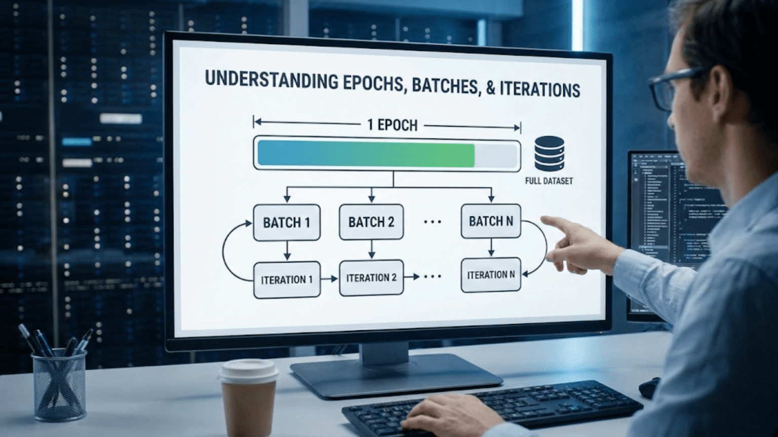
In deep learning training, an epoch is one complete pass through the entire training dataset, a batch is a subset of training examples processed together in one forward/backward pass, and an iteration is one update of the model’s parameters (processing one batch). For example, with 1,000 training examples and batch size 100, one epoch contains 10 iterations (10 batches of 100 examples each). Batch size affects training speed, memory usage, and model performance—larger batches train faster but require more memory and may generalize worse.
Introduction: The Vocabulary of Training
Imagine you’re studying for an exam using flashcards. You could study all 1,000 flashcards in one marathon session, or you could break them into manageable stacks of 50 cards, reviewing each stack multiple times, and cycling through all stacks several times before the exam. The way you organize your study sessions—how many cards per stack, how many times through each stack, how many full cycles through all cards—parallels how neural networks organize training.
Three fundamental terms describe neural network training: epochs, batches, and iterations. These aren’t just jargon—they represent critical decisions about how training proceeds. Set the batch size too large and you’ll run out of memory. Too small and training crawls. Too many epochs and you overfit. Too few and you underfit. Understanding these concepts is essential for effective training.
Yet these terms confuse many newcomers. What exactly is the difference between an iteration and an epoch? How does batch size affect training? Why do practitioners use mini-batches rather than processing the entire dataset at once? The answers involve tradeoffs between computational efficiency, memory constraints, and model performance.
This comprehensive guide clarifies epochs, batches, and iterations completely. You’ll learn precise definitions, the relationships between them, how to calculate training steps, how to choose batch size, the impact on training dynamics, practical examples, and best practices for configuring these fundamental training parameters.
Definitions: The Core Concepts
Let’s define each term precisely.
Epoch
Definition: One complete pass through the entire training dataset
Meaning:
- Model sees every training example exactly once
- All examples used for training (in some order)
- Completes one full cycle through data
Example:
Training dataset: 10,000 images

Epoch 1: Model processes all 10,000 images (once each)
Epoch 2: Model processes all 10,000 images again (once each)
Epoch 3: Model processes all 10,000 images again (once each)
...

After 100 epochs: Model has seen each image 100 timesWhy Multiple Epochs?:
- One pass rarely sufficient for learning
- Model improves with repeated exposure
- Typically train for 10-1000+ epochs
- Stop when validation performance plateaus
Batch
Definition: A subset of training examples processed together in one forward/backward pass
Meaning:
- Group of examples processed simultaneously
- Model makes predictions on batch
- Computes loss on batch
- Updates weights once per batch
Example:
Training dataset: 10,000 images
Batch size: 100 images

Batch 1: Images 1-100
Batch 2: Images 101-200
Batch 3: Images 201-300
...
Batch 100: Images 9,901-10,000

Total: 100 batchesTypes of Batches:
Full Batch (Batch Gradient Descent):
- Batch size = entire dataset
- Example: All 10,000 images in one batch
Mini-Batch (Mini-Batch Gradient Descent):
- Batch size = subset (typically 32-256)
- Example: Batches of 64 images
Single Example (Stochastic Gradient Descent):
- Batch size = 1
- Example: One image at a time
Iteration
Definition: One update of the model’s parameters (processing one batch)
Meaning:
- Process one batch through forward pass
- Compute gradients via backward pass
- Update weights once
- Equals one gradient descent step
Example:
One iteration:
1. Forward pass on batch → predictions
2. Compute loss
3. Backward pass → gradients
4. Update weights

Each batch processed = one iterationThe Relationship: How They Connect
Understanding the mathematical relationship is crucial.
The Formula
Number of Iterations per Epoch = Training Examples / Batch Size

Number of Iterations Total = (Training Examples / Batch Size) × Number of EpochsSimplified:
Iterations per Epoch = Dataset Size / Batch Size
Total Iterations = Iterations per Epoch × EpochsExample Calculations
Example 1:
Training examples: 1,000
Batch size: 50
Epochs: 10

Iterations per epoch = 1,000 / 50 = 20
Total iterations = 20 × 10 = 200

Interpretation:
- Each epoch: 20 weight updates (20 batches)
- Total training: 200 weight updatesExample 2:
Training examples: 60,000 (MNIST)
Batch size: 128
Epochs: 100

Iterations per epoch = 60,000 / 128 = 468.75 ≈ 469
Total iterations = 469 × 100 = 46,900

Interpretation:
- Each epoch: 469 weight updates
- Total training: 46,900 weight updatesExample 3:
Training examples: 1,000,000
Batch size: 256
Epochs: 50

Iterations per epoch = 1,000,000 / 256 = 3,906.25 ≈ 3,907
Total iterations = 3,907 × 50 = 195,350

Interpretation:
- Each epoch: ~3,907 weight updates
- Total training: ~195,000 weight updatesVisual Representation
Dataset: [Example 1, Example 2, Example 3, ..., Example 1000]

Batch Size = 100

┌─────────────── EPOCH 1 ───────────────────────────┐
│                                                   │
│ Iteration 1: [Examples 1-100]   → Update weights  │
│ Iteration 2: [Examples 101-200] → Update weights  │
│ Iteration 3: [Examples 201-300] → Update weights  │
│ ...                                               │
│ Iteration 10: [Examples 901-1000] → Update weights│
│                                                   │
└───────────────────────────────────────────────────┘
                    ↓
┌─────────────── EPOCH 2 ───────────────────────────┐
│                                                   │
│ Iteration 11: [Examples 1-100]   → Update weights │
│ Iteration 12: [Examples 101-200] → Update weights │
│ ...                                               │
│ Iteration 20: [Examples 901-1000] → Update weights│
│                                                   │
└───────────────────────────────────────────────────┘

And so on...Batch Size: The Critical Hyperparameter
Batch size significantly impacts training. Let’s explore its effects.
Small Batch Size (e.g., 8, 16, 32)
Advantages:
- Less memory: Can train larger models
- More updates: Faster initial progress
- Better generalization: Noise helps escape local minima
- Regularization effect: Acts as noise-based regularization
Disadvantages:
- Noisy gradients: High variance in updates
- Slower computation: Poor GPU utilization
- Longer wall-clock time: More iterations needed
- Less stable: Training can be erratic
Example:
Dataset: 10,000 examples
Batch size: 32

Iterations per epoch: 312
→ 312 weight updates per epoch
→ Lots of updates, but each is noisyWhen to Use:
- Limited GPU memory
- Small datasets
- When want regularization effect
- Experimenting/prototyping
Large Batch Size (e.g., 256, 512, 1024+)
Advantages:
- Stable gradients: Low variance in updates
- Faster computation: Better GPU utilization
- Fewer iterations: Faster per epoch
- Smoother convergence: More predictable
Disadvantages:
- High memory: May not fit in GPU
- Worse generalization: Can get stuck in sharp minima
- Fewer updates: Slower initial learning
- May need adjustment: Learning rate, epochs
Example:
Dataset: 10,000 examples
Batch size: 1,000

Iterations per epoch: 10
→ Only 10 weight updates per epoch
→ Each update very stable, but fewer updatesWhen to Use:
- Large datasets
- Ample GPU memory
- Production training (speed matters)
- When have tuned learning rate appropriately
Sweet Spot: 32-256
Most Common: Batch sizes 32, 64, 128, 256
Why:
- Balance of stability and updates
- Efficient GPU utilization
- Good generalization
- Widely tested defaults
General Guidelines:
Computer Vision (images): 32-128
Natural Language Processing: 32-64
Tabular data: 32-256
Reinforcement Learning: Varies widely

Default starting point: 32 or 64
Powers of 2
Common Pattern: Batch sizes are powers of 2
Why:
- GPU/TPU memory alignment
- Efficient matrix operations
- Historical convention
- Slightly better performance
Common Values: 8, 16, 32, 64, 128, 256, 512, 1024
Impact on Training Dynamics
Batch size affects how training proceeds.
Gradient Noise
Small Batches:
Gradient estimated from few examples
High variance
Batch 1: Gradient points direction A
Batch 2: Gradient points direction B
Noisy but helps explorationLarge Batches:
Gradient estimated from many examples
Low variance
All batches: Gradient points similar direction
Stable but may miss good solutionsVisualization:
Loss Landscape

Small batch path:  •→←•→←•→• (wiggly, explores)
Large batch path:  •→→→→→→• (straight, direct)
                        ↓
Both reach minimum, different pathsLearning Rate Relationship
Linear Scaling Rule: When increasing batch size, increase learning rate proportionally
Example:
Batch size 32, Learning rate 0.001: Works well

Increase batch size to 256 (8x larger):
Should increase learning rate to 0.008 (8x larger)

Reasoning: Larger batches give more stable gradients
Can take larger steps without instabilityNot Always Perfect: May need experimentation
Generalization
Empirical Finding: Smaller batches often generalize better
Sharp vs. Flat Minima:
Sharp Minimum:
    Loss
     │  ╱‾╲  ← Narrow valley
     │ ╱   ╲
     │╱     ╲

Flat Minimum:
    Loss
     │  ╱‾‾‾╲ ← Wide valley
     │ ╱     ╲
     │╱       ╲

Large batches → Sharp minima (worse generalization)
Small batches → Flat minima (better generalization)Intuition:
- Small batch noise helps escape sharp minima
- Finds solutions robust to perturbations
- Better performance on test data
Training Time
Wall-Clock Time = (Iterations per Epoch) × (Time per Iteration) × (Epochs)
Tradeoff:
Small batch (32):
- More iterations per epoch: 312
- Fast time per iteration: 0.01s
- Total per epoch: 3.12s

Large batch (512):
- Fewer iterations per epoch: 19
- Slower time per iteration: 0.05s
- Total per epoch: 0.95s

Large batch trains faster (wall-clock time)But: Large batch may need more epochs for same performance
Choosing Epochs
How many times through the dataset?
Too Few Epochs
Problem: Underfitting, model hasn’t learned enough
Symptoms:
Epoch 1: Train loss=0.8, Val loss=0.82
Epoch 5: Train loss=0.5, Val loss=0.53
Epoch 10: Train loss=0.3, Val loss=0.35

Both still decreasing → Stop too early
Model could improve moreSolution: Train longer
Too Many Epochs
Problem: Overfitting, memorizing training data
Symptoms:
Epoch 1: Train=0.8, Val=0.82
Epoch 50: Train=0.1, Val=0.25
Epoch 100: Train=0.01, Val=0.35

Training keeps improving, validation gets worse
Clear overfittingSolution: Stop earlier, use early stopping
Just Right
Sweet Spot: Validation loss minimized
Example:
Epoch 1: Train=0.8, Val=0.82
Epoch 30: Train=0.2, Val=0.24
Epoch 50: Train=0.15, Val=0.22 ← Best validation
Epoch 70: Train=0.1, Val=0.25

Best to stop around epoch 50Early Stopping
Automatic Solution: Stop when validation stops improving
Algorithm:
patience = 10  # Wait 10 epochs for improvement

best_val_loss = infinity
epochs_no_improve = 0

for epoch in range(max_epochs):
    train()
    val_loss = validate()

    if val_loss < best_val_loss:
        best_val_loss = val_loss
        epochs_no_improve = 0
        save_model()
    else:
        epochs_no_improve += 1

    if epochs_no_improve >= patience:
        print("Early stopping!")
        break

restore_best_model()Benefits:
- Automatic
- Prevents overfitting
- Saves time
Practical Examples
Example 1: MNIST Digit Classification
Dataset: 60,000 training images
Configuration:
Batch size: 128
Epochs: 10

Calculations:
Iterations per epoch = 60,000 / 128 = 468.75 ≈ 469
Total iterations = 469 × 10 = 4,690

Training process:
Epoch 1: 469 iterations (469 weight updates)
Epoch 2: 469 iterations
...
Epoch 10: 469 iterations

Total: 4,690 weight updatesTraining Log:
Epoch 1/10 - 469/469 batches - loss: 0.3521 - val_loss: 0.2012
Epoch 2/10 - 469/469 batches - loss: 0.1823 - val_loss: 0.1456
Epoch 3/10 - 469/469 batches - loss: 0.1345 - val_loss: 0.1201
...Example 2: ImageNet
Dataset: 1,281,167 training images
Configuration:
Batch size: 256
Epochs: 90

Calculations:
Iterations per epoch = 1,281,167 / 256 = 5,004.56 ≈ 5,005
Total iterations = 5,005 × 90 = 450,450

Training process:
Each epoch: 5,005 iterations
Total: 450,450 weight updates
Time: Days to weeks on GPUExample 3: Custom Dataset
Dataset: 5,000 examples
Small Batch Experiment:
Batch size: 16
Epochs: 100

Iterations per epoch = 5,000 / 16 = 312.5 ≈ 313
Total iterations = 313 × 100 = 31,300

Many updates, longer trainingLarge Batch Experiment:
Batch size: 256
Epochs: 100

Iterations per epoch = 5,000 / 256 = 19.53 ≈ 20
Total iterations = 20 × 100 = 2,000

Fewer updates, faster trainingImplementation Examples
Keras/TensorFlow
import tensorflow as tf
from tensorflow import keras

# Load data
(X_train, y_train), (X_val, y_val) = keras.datasets.mnist.load_data()

# Preprocess
X_train = X_train.reshape(-1, 784) / 255.0
X_val = X_val.reshape(-1, 784) / 255.0

# Model
model = keras.Sequential([
    keras.layers.Dense(128, activation='relu'),
    keras.layers.Dense(10, activation='softmax')
])

model.compile(optimizer='adam', loss='sparse_categorical_crossentropy',
              metrics=['accuracy'])

# Training configuration
batch_size = 64
epochs = 10

# Calculate iterations
train_size = len(X_train)
iterations_per_epoch = train_size // batch_size
total_iterations = iterations_per_epoch * epochs

print(f"Training examples: {train_size}")
print(f"Batch size: {batch_size}")
print(f"Iterations per epoch: {iterations_per_epoch}")
print(f"Total iterations: {total_iterations}")

# Train
history = model.fit(
    X_train, y_train,
    batch_size=batch_size,
    epochs=epochs,
    validation_data=(X_val, y_val),
    verbose=1
)

# Output:
# Training examples: 60000
# Batch size: 64
# Iterations per epoch: 937
# Total iterations: 9370
#
# Epoch 1/10
# 937/937 [==============================] - 2s 2ms/step - loss: 0.2912
# ...PyTorch
import torch
import torch.nn as nn
from torch.utils.data import DataLoader, TensorDataset

# Data
X_train = torch.randn(10000, 20)
y_train = torch.randint(0, 2, (10000,))

# Dataset and DataLoader
dataset = TensorDataset(X_train, y_train)
batch_size = 128
dataloader = DataLoader(dataset, batch_size=batch_size, shuffle=True)

# Model
model = nn.Sequential(
    nn.Linear(20, 64),
    nn.ReLU(),
    nn.Linear(64, 2)
)

optimizer = torch.optim.Adam(model.parameters())
criterion = nn.CrossEntropyLoss()

# Training configuration
epochs = 10
train_size = len(dataset)
iterations_per_epoch = len(dataloader)
total_iterations = iterations_per_epoch * epochs

print(f"Training examples: {train_size}")
print(f"Batch size: {batch_size}")
print(f"Iterations per epoch: {iterations_per_epoch}")
print(f"Total iterations: {total_iterations}")

# Training loop
iteration = 0
for epoch in range(epochs):
    for batch_idx, (X_batch, y_batch) in enumerate(dataloader):
        # Forward pass
        outputs = model(X_batch)
        loss = criterion(outputs, y_batch)

        # Backward pass
        optimizer.zero_grad()
        loss.backward()
        optimizer.step()

        iteration += 1

        if batch_idx % 20 == 0:
            print(f"Epoch {epoch+1}/{epochs}, "
                  f"Batch {batch_idx}/{iterations_per_epoch}, "
                  f"Iteration {iteration}/{total_iterations}, "
f"Loss: {loss.item():.4f}")Custom Training Loop with Progress Tracking
import numpy as np

def train_with_progress(model, X_train, y_train, batch_size=32, epochs=10):
    """Training with detailed progress tracking"""
    n_samples = len(X_train)
    n_batches = int(np.ceil(n_samples / batch_size))
    total_iterations = n_batches * epochs

    print(f"Training Configuration:")
    print(f"  Samples: {n_samples}")
    print(f"  Batch size: {batch_size}")
    print(f"  Epochs: {epochs}")
    print(f"  Batches per epoch: {n_batches}")
    print(f"  Total iterations: {total_iterations}\n")

    global_iteration = 0

    for epoch in range(epochs):
        # Shuffle data
        indices = np.random.permutation(n_samples)
        X_shuffled = X_train[indices]
        y_shuffled = y_train[indices]

        epoch_loss = 0

        for batch_idx in range(n_batches):
            # Get batch
            start = batch_idx * batch_size
            end = min(start + batch_size, n_samples)
            X_batch = X_shuffled[start:end]
            y_batch = y_shuffled[start:end]

            # Train on batch
            loss = model.train_step(X_batch, y_batch)
            epoch_loss += loss

            global_iteration += 1

            # Progress
            if batch_idx % 50 == 0:
                progress = (batch_idx / n_batches) * 100
                print(f"Epoch {epoch+1}/{epochs} - "
                      f"Batch {batch_idx}/{n_batches} ({progress:.0f}%) - "
                      f"Global Iteration {global_iteration}/{total_iterations} - "
                      f"Loss: {loss:.4f}")

        # Epoch summary
        avg_loss = epoch_loss / n_batches
print(f"Epoch {epoch+1} complete - Avg Loss: {avg_loss:.4f}\n")Common Pitfalls and Solutions
Pitfall 1: Batch Size Doesn’t Divide Dataset Evenly
Problem:
Dataset: 1,000 examples
Batch size: 64

1,000 / 64 = 15.625 (not even)Solutions:
Drop Last Batch (Incomplete):
# PyTorch
dataloader = DataLoader(dataset, batch_size=64, drop_last=True)
# Uses 15 batches, drops last 40 examplesKeep Last Batch (Smaller):
# Default behavior
# 15 batches of 64, 1 batch of 40Pad Last Batch:
# Pad with zeros or repeat examples
# All batches size 64Pitfall 2: Out of Memory
Problem: Batch size too large for GPU
Symptoms:
RuntimeError: CUDA out of memorySolutions:
- Reduce batch size: 128 → 64 → 32
- Gradient accumulation: Simulate large batch
- Use smaller model: Fewer parameters
- Use mixed precision: FP16 instead of FP32
Pitfall 3: Training Too Long
Problem: Overfitting from too many epochs
Solution: Early stopping (discussed above)
Pitfall 4: Inconsistent Batch Sizes
Problem: Last batch different size affects batch normalization
Solution:
# Drop last incomplete batch
dataloader = DataLoader(..., drop_last=True)Best Practices
1. Start with Common Values
Batch size: 32 or 64
Epochs: 10-100 (use early stopping)Adjust based on results.
2. Monitor Training
# Track loss per epoch
# Watch for:
# - Steady decrease (good)
# - Plateau (may need more epochs or different learning rate)
# - Divergence (reduce learning rate or batch size)3. Use Early Stopping
early_stop = keras.callbacks.EarlyStopping(
    monitor='val_loss',
    patience=10,
    restore_best_weights=True
)4. Adjust Learning Rate with Batch Size
# If increasing batch size 4x
# Consider increasing learning rate 4x
# (Linear scaling rule)5. Powers of 2 for Batch Size
Prefer: 32, 64, 128, 256
Over: 30, 50, 100, 200Comparison Table
| Aspect | Small Batch (32) | Medium Batch (128) | Large Batch (512) |
|---|---|---|---|
| Memory Usage | Low | Medium | High |
| Iterations/Epoch | Many | Medium | Few |
| Gradient Noise | High | Medium | Low |
| Training Stability | Noisy | Balanced | Stable |
| Generalization | Better | Good | May be worse |
| Computation Speed | Slower | Balanced | Faster |
| GPU Utilization | Poor | Good | Excellent |
| Learning Rate | Standard | May need adjustment | Need to increase |
| Best For | Small GPUs, experimentation | General use | Large datasets, production |
Conclusion: Orchestrating Training
Epochs, batches, and iterations are the fundamental units that structure neural network training. Understanding them transforms training from a black box into a transparent process you can reason about and optimize.
Epochs determine how many times the model sees the complete dataset, balancing learning thoroughness against overfitting risk. Too few and the model hasn’t learned enough; too many and it memorizes training data.
Batch size controls how many examples process together, creating a crucial tradeoff between computational efficiency, memory usage, gradient stability, and generalization. The sweet spot of 32-256 balances these factors for most applications.
Iterations count the actual parameter updates, directly determining training progress. More iterations generally mean better training, up to the point of overfitting.
The relationships between these concepts determine training dynamics:
- Smaller batches mean more iterations per epoch and noisier but potentially better-generalizing updates
- Larger batches mean fewer iterations per epoch and stabler but potentially worse-generalizing updates
- More epochs mean more total iterations but risk overfitting
- Early stopping automatically finds the right number of epochs
As you train models, remember that these aren’t just abstract concepts—they’re practical levers controlling how training proceeds. Start with standard values (batch size 32-64, epochs until early stopping), monitor training curves, and adjust based on what you observe. With experience, you’ll develop intuition for the right configuration for different problems.
Master epochs, batches, and iterations, and you’ve mastered the fundamental rhythm of neural network training—the organized, iterative process by which random weights become learned representations that solve real problems.