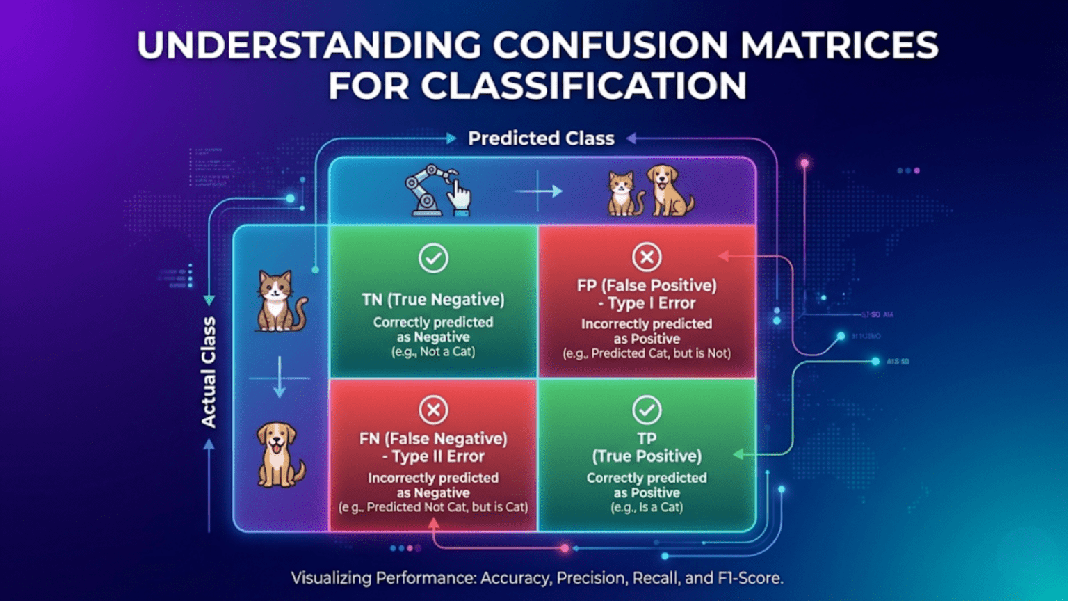
A confusion matrix is a table that summarizes a classification model’s performance by counting how many predictions fell into each combination of predicted and actual class. For binary classification, it has four cells: True Negatives (TN), False Positives (FP), False Negatives (FN), and True Positives (TP). From these four numbers, every classification metric — accuracy, precision, recall, F1 score, specificity — can be derived. The confusion matrix is the single most informative snapshot of a classifier’s behavior, revealing not just overall performance but the specific types of errors the model makes.
Introduction: The Full Picture of Classification Performance
A model achieves 95% accuracy on a medical test for a rare disease that affects 5% of the population. Impressive? Not if the model predicts “healthy” for everyone — it achieves exactly 95% accuracy while catching zero actual cases.
This is why accuracy alone never tells the full story of a classifier’s performance. To truly understand what a model is doing, you need to see how it handles every combination of actual class and predicted class. A single number collapses all of that nuance into one statistic, hiding critical information about which types of errors the model is making.
The confusion matrix solves this problem by making the full picture explicit. For every possible combination of true label and predicted label, it records a count. With four cells for binary classification — or n² cells for n-class problems — the confusion matrix reveals whether a model catches the cases it’s supposed to catch, whether it raises too many false alarms, whether it consistently confuses specific class pairs, and where exactly its mistakes are concentrated.
Every classification metric worth knowing — accuracy, precision, recall, specificity, F1 score, Matthews Correlation Coefficient, and more — derives from the confusion matrix. Understanding the matrix means understanding all the metrics that flow from it, and understanding why each one emphasizes different aspects of performance.
This comprehensive guide covers confusion matrices completely. You’ll learn the four fundamental cells of binary classification, every derived metric with intuitive interpretations, how to read and construct confusion matrices in Python, multi-class confusion matrices, normalized variants, visualizations, and practical guidance on what to look for in your own model evaluations.
The Binary Confusion Matrix
The Four Cells
For binary classification with classes 0 (negative) and 1 (positive):
                    PREDICTED
                  Negative (0)    Positive (1)
ACTUAL  Neg (0)  True Negative   False Positive
        Pos (1)  False Negative  True Positive

Abbreviated:
                  Predicted 0     Predicted 1
Actual 0          TN              FP
Actual 1 FN TPEach cell defined:
True Negative (TN):
Actual: Negative (0)
Predicted: Negative (0)
Correct rejection — model correctly said "no"

Example (spam filter): Legitimate email → "Not Spam" ✓
Example (disease test): Healthy patient → "Negative" ✓False Positive (FP) — Type I Error:
Actual: Negative (0)
Predicted: Positive (1)
False alarm — model incorrectly said "yes"

Example (spam filter): Legitimate email → "Spam" ✗
Example (disease test): Healthy patient → "Positive" ✗
Also called: Type I Error, False Alarm, False DiscoveryFalse Negative (FN) — Type II Error:
Actual: Positive (1)
Predicted: Negative (0)
Miss — model incorrectly said "no"

Example (spam filter): Spam email → "Not Spam" ✗
Example (disease test): Sick patient → "Negative" ✗
Also called: Type II Error, Missed Detection, False DismissalTrue Positive (TP):
Actual: Positive (1)
Predicted: Positive (1)
Correct detection — model correctly said "yes"

Example (spam filter): Spam email → "Spam" ✓
Example (disease test): Sick patient → "Positive" ✓A Concrete Numerical Example
Problem: Email spam classifier tested on 1,000 emails
                    Predicted: Ham    Predicted: Spam
Actual: Ham (400)       380 (TN)          20 (FP)
Actual: Spam (600)       60 (FN)         540 (TP)

TN = 380  (correctly flagged as legitimate)
FP =  20  (legitimate emails incorrectly flagged as spam)
FN =  60  (spam emails that slipped through)
TP = 540  (spam correctly caught)

Total examples: 380 + 20 + 60 + 540 = 1,000 ✓Reading the matrix:
Row 1 (Actual Ham):   380 + 20  = 400 total actual ham emails
Row 2 (Actual Spam):  60 + 540 = 600 total actual spam emails
Col 1 (Pred Ham):     380 + 60  = 440 total predicted as ham
Col 2 (Pred Spam): 20 + 540 = 560 total predicted as spamEvery Metric Derived from the Confusion Matrix
Once you have TN, FP, FN, TP, every classification metric follows algebraically.
Core Metrics
Accuracy:
Accuracy = (TP + TN) / (TP + TN + FP + FN)
         = (540 + 380) / 1000
         = 920 / 1000 = 0.92 (92%)

"What fraction of all predictions were correct?"

Limitation: Misleading with class imbalance.Precision (Positive Predictive Value):
Precision = TP / (TP + FP)
          = 540 / (540 + 20)
          = 540 / 560 = 0.964 (96.4%)

"Of all emails flagged as spam, what fraction were actually spam?"
High precision → few false alarms (legitimate email rarely blocked)
Low precision → many false alarms (inbox disrupted)Recall (Sensitivity / True Positive Rate):
Recall = TP / (TP + FN)
       = 540 / (540 + 60)
       = 540 / 600 = 0.90 (90%)

"Of all actual spam emails, what fraction did we catch?"
High recall → few spam emails slip through
Low recall → much spam reaches inboxSpecificity (True Negative Rate):
Specificity = TN / (TN + FP)
            = 380 / (380 + 20)
            = 380 / 400 = 0.95 (95%)

"Of all actual legitimate emails, what fraction were correctly passed?"
High specificity → few legitimate emails blocked
Complement of False Positive Rate: Specificity = 1 − FPRFalse Positive Rate (FPR):
FPR = FP / (FP + TN)
    = 20 / (20 + 380)
    = 20 / 400 = 0.05 (5%)

"Of all actual negatives, what fraction did we incorrectly flag?"
Used in ROC curve construction (x-axis).False Negative Rate (FNR) / Miss Rate:
FNR = FN / (FN + TP)
    = 60 / (60 + 540)
    = 60 / 600 = 0.10 (10%)

Complement of recall: FNR = 1 − RecallF1 Score:
F1 = 2 × (Precision × Recall) / (Precision + Recall)
   = 2 × (0.964 × 0.90) / (0.964 + 0.90)
   = 2 × 0.868 / 1.864
   = 0.931 (93.1%)

Harmonic mean of precision and recall.
Better than accuracy for imbalanced classes.Matthews Correlation Coefficient (MCC):
MCC = (TP×TN − FP×FN) / √[(TP+FP)(TP+FN)(TN+FP)(TN+FN)]
    = (540×380 − 20×60) / √[(560)(600)(400)(440)]
    = (205,200 − 1,200) / √[59,136,000,000]
    = 204,000 / 243,180
    = 0.839

Range: −1 to +1
+1: Perfect classifier
 0: No better than random
−1: Perfectly inverted

Most informative single metric for imbalanced classification.
Unlike F1, accounts for all four confusion matrix cells.Balanced Accuracy:
Balanced Accuracy = (Recall + Specificity) / 2
                  = (0.90 + 0.95) / 2
                  = 0.925

Better than accuracy when classes are imbalanced.
Average of recall per class — each class contributes equally.All Metrics from the Spam Example
Metric                  Value    Interpretation
────────────────────────────────────────────────────────────────
Accuracy                92.0%    92% of all predictions correct
Precision               96.4%    96.4% of flagged emails are spam
Recall (Sensitivity)    90.0%    90% of spam caught
Specificity             95.0%    95% of ham correctly passed
FPR                      5.0%    5% of ham incorrectly blocked
FNR                     10.0%    10% of spam slips through
F1 Score                93.1%    Balanced precision/recall
MCC                     0.839    Strong positive correlation
Balanced Accuracy 92.5% Average of recall + specificityThe Precision-Recall Tradeoff Visualized Through the Matrix
Changing the decision threshold shifts values within the confusion matrix, creating the precision-recall tradeoff.
Lower threshold (predict spam more aggressively):
  More emails flagged as spam
  TP increases (catch more real spam)     → Recall ↑
  FP increases (more ham blocked)         → Precision ↓

                  Pred Ham    Pred Spam
  Actual Ham         340          60    ← More FP
  Actual Spam         20         580    ← More TP
  Precision = 580/(580+60) = 90.6%  ↓ (was 96.4%)
  Recall    = 580/(580+20) = 96.7%  ↑ (was 90.0%)

Raise threshold (predict spam more conservatively):
  Fewer emails flagged as spam
  TP decreases (miss more real spam)      → Recall ↓
  FP decreases (less ham blocked)         → Precision ↑

                  Pred Ham    Pred Spam
  Actual Ham         395           5    ← Fewer FP
  Actual Spam        120         480    ← Fewer TP
  Precision = 480/(480+5) = 99.0%  ↑ (was 96.4%)
Recall = 480/(480+120) = 80.0% ↓ (was 90.0%)This is the fundamental tradeoff: you cannot simultaneously maximize precision and recall. The confusion matrix makes the mechanism visible.
Python Implementation
Building and Visualizing Confusion Matrices
import numpy as np
import pandas as pd
import matplotlib.pyplot as plt
import matplotlib.colors as mcolors
from sklearn.datasets import load_breast_cancer, load_iris
from sklearn.model_selection import train_test_split
from sklearn.preprocessing import StandardScaler
from sklearn.linear_model import LogisticRegression
from sklearn.metrics import (confusion_matrix, ConfusionMatrixDisplay,
                              classification_report, accuracy_score,
                              precision_score, recall_score, f1_score,
                              matthews_corrcoef, balanced_accuracy_score,
                              roc_auc_score)
from sklearn.pipeline import Pipeline

# ── Dataset and model ───────────────────────────────────────────
cancer  = load_breast_cancer()
X, y    = cancer.data, cancer.target
names   = list(cancer.target_names)

X_train, X_test, y_train, y_test = train_test_split(
    X, y, test_size=0.2, random_state=42, stratify=y
)

pipe = Pipeline([
    ('scaler', StandardScaler()),
    ('clf',    LogisticRegression(C=1.0, max_iter=1000, random_state=42))
])
pipe.fit(X_train, y_train)
y_pred  = pipe.predict(X_test)
y_proba = pipe.predict_proba(X_test)[:, 1]Extracting All Four Values
# Method 1: sklearn confusion_matrix
cm = confusion_matrix(y_test, y_pred)
print("Raw confusion matrix:")
print(cm)
print(f"Shape: {cm.shape}")

# Method 2: Unpack TN, FP, FN, TP directly
tn, fp, fn, tp = confusion_matrix(y_test, y_pred).ravel()
print(f"\nTN={tn}  FP={fp}")
print(f"FN={fn}  TP={tp}")

# Method 3: Manual computation
total   = len(y_test)
correct = (y_pred == y_test).sum()
print(f"\nTotal: {total}, Correct: {correct}, Wrong: {total-correct}")Computing Every Metric
def full_confusion_metrics(y_true, y_pred, y_proba=None,
                            pos_label=1):
    """
    Compute every metric derivable from the confusion matrix.
    Returns a formatted report and a dict of values.
    """
    cm          = confusion_matrix(y_true, y_pred, labels=[0, 1])
    tn, fp, fn, tp = cm.ravel()
    total       = tn + fp + fn + tp

    # Core counts
    metrics = {
        'TN': tn, 'FP': fp, 'FN': fn, 'TP': tp,
        'Total': total,
        'Actual Pos': tp + fn,
        'Actual Neg': tn + fp,
        'Pred Pos':   tp + fp,
        'Pred Neg':   tn + fn,
    }

    # Rates
    eps = 1e-9  # prevent division by zero
    metrics.update({
        'Accuracy':           (tp + tn) / (total + eps),
        'Precision':           tp / (tp + fp + eps),
        'Recall':              tp / (tp + fn + eps),
        'Specificity':         tn / (tn + fp + eps),
        'FPR':                 fp / (fp + tn + eps),
        'FNR':                 fn / (fn + tp + eps),
        'F1':                  f1_score(y_true, y_pred),
        'Balanced Accuracy':   balanced_accuracy_score(y_true, y_pred),
        'MCC':                 matthews_corrcoef(y_true, y_pred),
    })

    if y_proba is not None:
        metrics['ROC-AUC'] = roc_auc_score(y_true, y_proba)

    # Print report
    print("=" * 52)
    print("  CONFUSION MATRIX METRICS")
    print("=" * 52)
    print(f"\n  Confusion Matrix:")
    print(f"    TN={tn:5d}   FP={fp:5d}")
    print(f"    FN={fn:5d}   TP={tp:5d}")
    print(f"\n  Class Counts:")
    print(f"    Actual Positive:    {tp+fn:5d}")
    print(f"    Actual Negative:    {tn+fp:5d}")
    print(f"    Predicted Positive: {tp+fp:5d}")
    print(f"    Predicted Negative: {tn+fn:5d}")
    print(f"\n  Performance Metrics:")
    print(f"    Accuracy:           {metrics['Accuracy']:.4f}")
    print(f"    Precision:          {metrics['Precision']:.4f}")
    print(f"    Recall:             {metrics['Recall']:.4f}")
    print(f"    Specificity:        {metrics['Specificity']:.4f}")
    print(f"    FPR:                {metrics['FPR']:.4f}")
    print(f"    FNR:                {metrics['FNR']:.4f}")
    print(f"    F1 Score:           {metrics['F1']:.4f}")
    print(f"    Balanced Accuracy:  {metrics['Balanced Accuracy']:.4f}")
    print(f"    MCC:                {metrics['MCC']:.4f}")
    if 'ROC-AUC' in metrics:
        print(f"    ROC-AUC:            {metrics['ROC-AUC']:.4f}")
    print("=" * 52)

    return metrics

results = full_confusion_metrics(y_test, y_pred, y_proba)Expected Output:
====================================================
  CONFUSION MATRIX METRICS
====================================================
  Confusion Matrix:
    TN=   39   FP=    2
    FN=    1   TP=   72

  Class Counts:
    Actual Positive:       73
    Actual Negative:       41
    Predicted Positive:    74
    Predicted Negative:    40

  Performance Metrics:
    Accuracy:           0.9737
    Precision:          0.9730
    Recall:             0.9863
    Specificity:        0.9512
    FPR:                0.0488
    FNR:                0.0137
    F1 Score:           0.9796
    Balanced Accuracy:  0.9687
    MCC:                0.9431
    ROC-AUC:            0.9975
====================================================Visualization Suite
fig, axes = plt.subplots(2, 2, figsize=(13, 11))

# ── 1. Standard confusion matrix ────────────────────────────────
ax = axes[0, 0]
disp = ConfusionMatrixDisplay(
    confusion_matrix(y_test, y_pred),
    display_labels=names
)
disp.plot(ax=ax, colorbar=False, cmap='Blues')
ax.set_title('Confusion Matrix (Raw Counts)', fontsize=12)

# Add percentage annotations
cm_raw = confusion_matrix(y_test, y_pred)
total  = cm_raw.sum()
for i in range(2):
    for j in range(2):
        pct = cm_raw[i, j] / total * 100
        ax.text(j, i + 0.35, f'({pct:.1f}%)',
                ha='center', va='center',
                fontsize=9, color='gray')

# ── 2. Normalized confusion matrix (by true class) ─────────────
ax = axes[0, 1]
cm_norm = confusion_matrix(y_test, y_pred, normalize='true')
disp_n  = ConfusionMatrixDisplay(cm_norm, display_labels=names)
disp_n.plot(ax=ax, colorbar=False, cmap='Blues',
            values_format='.3f')
ax.set_title('Confusion Matrix (Normalized by True Class)\n'
             '= Recall per class on diagonal', fontsize=11)

# ── 3. Metrics bar chart ────────────────────────────────────────
ax = axes[1, 0]
metric_names = ['Accuracy', 'Precision', 'Recall',
                'Specificity', 'F1', 'Balanced\nAccuracy', 'MCC']
metric_vals  = [
    results['Accuracy'], results['Precision'],
    results['Recall'],   results['Specificity'],
    results['F1'],       results['Balanced Accuracy'],
    results['MCC']
]
colors_bar = ['steelblue' if v >= 0.95 else
              'coral'     if v < 0.90  else
              'gold'      for v in metric_vals]

bars = ax.barh(metric_names, metric_vals, color=colors_bar,
               edgecolor='white', height=0.6)
ax.set_xlim(0, 1.08)
ax.axvline(0.9,  color='gray',  linestyle='--', alpha=0.5,
           linewidth=1, label='0.90')
ax.axvline(0.95, color='green', linestyle='--', alpha=0.5,
           linewidth=1, label='0.95')
for bar, val in zip(bars, metric_vals):
    ax.text(val + 0.005, bar.get_y() + bar.get_height()/2,
            f'{val:.4f}', va='center', fontsize=9)
ax.set_title('All Metrics at a Glance', fontsize=12)
ax.legend(fontsize=9)
ax.grid(True, alpha=0.2, axis='x')

# ── 4. Error type breakdown ─────────────────────────────────────
ax   = axes[1, 1]
vals = [tn, fp, fn, tp]
lbls = ['True\nNegative\n(TN)', 'False\nPositive\n(FP)',
        'False\nNegative\n(FN)', 'True\nPositive\n(TP)']
clrs = ['#2196F3', '#FF5722', '#FF9800', '#4CAF50']

wedges, texts, autotexts = ax.pie(
    vals, labels=lbls, colors=clrs,
    autopct='%1.1f%%', startangle=140,
    pctdistance=0.75,
    wedgeprops=dict(width=0.6, edgecolor='white', linewidth=2)
)
for autotext in autotexts:
    autotext.set_fontsize(10)
ax.set_title(f'Prediction Breakdown\n'
             f'(TN={tn}, FP={fp}, FN={fn}, TP={tp})', fontsize=11)

plt.suptitle('Confusion Matrix Analysis — Breast Cancer Classifier',
             fontsize=14, fontweight='bold')
plt.tight_layout()
plt.show()Normalized Confusion Matrices
Raw counts depend on dataset size and class balance. Normalization makes matrices comparable.
Three Normalization Modes
fig, axes = plt.subplots(1, 3, figsize=(16, 5))
norm_modes = [None, 'true', 'pred', 'all']
titles = [
    'Raw Counts',
    "Normalized by True\n(diagonal = Recall per class)",
    "Normalized by Predicted\n(diagonal = Precision per class)",
    "Normalized by All\n(proportion of total)"
]

for ax, norm, title in zip(axes, ['', 'true', 'pred'], titles):
    if norm == '':
        cm_plot = confusion_matrix(y_test, y_pred)
        fmt = 'd'
    else:
        cm_plot = confusion_matrix(y_test, y_pred, normalize=norm)
        fmt = '.3f'

    disp = ConfusionMatrixDisplay(cm_plot, display_labels=names)
    disp.plot(ax=ax, colorbar=False, cmap='Blues', values_format=fmt)
    ax.set_title(title, fontsize=10)

plt.suptitle('Three Ways to Display a Confusion Matrix',
             fontsize=13, fontweight='bold')
plt.tight_layout()
plt.show()

# Which to use:
print("When to use each normalization:")
print("  Raw counts:          When absolute errors matter")
print("  Normalize='true':   When recall per class matters (imbalanced data)")
print("  Normalize='pred':   When precision per class matters")
print(" Normalize='all': When overall proportion matters (rare: use raw)")Multi-Class Confusion Matrices
For n > 2 classes, the confusion matrix extends to n × n.
Reading a Multi-Class Matrix
# Iris dataset: 3 classes
iris    = load_iris()
X_ir, y_ir = iris.data, iris.target
ir_names   = list(iris.target_names)

X_tr_ir, X_te_ir, y_tr_ir, y_te_ir = train_test_split(
    X_ir, y_ir, test_size=0.3, stratify=y_ir, random_state=42
)

pipe_ir = Pipeline([
    ('scaler', StandardScaler()),
    ('clf',    LogisticRegression(max_iter=1000, random_state=42))
])
pipe_ir.fit(X_tr_ir, y_tr_ir)
y_pred_ir = pipe_ir.predict(X_te_ir)

cm_ir = confusion_matrix(y_te_ir, y_pred_ir)

print("3-Class Confusion Matrix (Iris):")
print(f"\n{'':12s} {'Pred: Setosa':>13} {'Pred: Versicolor':>17} "
      f"{'Pred: Virginica':>16}")
print("-" * 60)
for i, name in enumerate(ir_names):
    row = cm_ir[i]
print(f"True: {name:10s} {row[0]:>13d} {row[1]:>17d} {row[2]:>16d}")Output:
3-Class Confusion Matrix (Iris):

             Pred: Setosa   Pred: Versicolor   Pred: Virginica
------------------------------------------------------------
True: setosa            15                0                 0
True: versicolor         0               14                 1
True: virginica          0                2                13
Reading this matrix:
Diagonal (top-left to bottom-right): Correct predictions
  Setosa:     15/15 correct   (100%)
  Versicolor: 14/15 correct    (93%)
  Virginica:  13/15 correct    (87%)

Off-diagonal: Errors
  1 Versicolor predicted as Virginica
  2 Virginica predicted as Versicolor
(These two classes are the hardest to separate — biologically similar)Per-Class Metrics from Multi-Class Matrix
# scikit-learn classification_report handles multi-class automatically
print(classification_report(y_te_ir, y_pred_ir, target_names=ir_names))Output:
              precision    recall  f1-score   support

      setosa       1.00      1.00      1.00        15
  versicolor       0.88      0.93      0.90        15
   virginica       0.93      0.87      0.90        15

    accuracy                           0.93        45
   macro avg       0.93      0.93      0.93        45
weighted avg 0.93 0.93 0.93 45How Per-Class Metrics Work in Multi-Class
# For each class c in a multi-class problem:
# Treat class c as "positive" and all others as "negative"
# Then compute TN, FP, FN, TP as in binary case

# Example for class "versicolor" (index 1):
# TP = correctly predicted versicolor
# FP = other classes predicted as versicolor
# FN = versicolor predicted as other classes
# TN = non-versicolor correctly predicted as non-versicolor

def per_class_metrics(cm, class_names):
    """Compute binary metrics for each class using OvR strategy."""
    n = len(class_names)
    print(f"\n{'Class':12s} {'TP':>5} {'FP':>5} {'FN':>5} {'TN':>5} "
          f"{'Prec':>7} {'Rec':>7} {'F1':>7}")
    print("-" * 60)

    for i, name in enumerate(class_names):
        tp = cm[i, i]
        fp = cm[:, i].sum() - tp      # Column sum minus diagonal
        fn = cm[i, :].sum() - tp      # Row sum minus diagonal
        tn = cm.sum() - tp - fp - fn

        prec = tp / (tp + fp + 1e-9)
        rec  = tp / (tp + fn + 1e-9)
        f1   = 2 * prec * rec / (prec + rec + 1e-9)

        print(f"{name:12s} {tp:>5} {fp:>5} {fn:>5} {tn:>5} "
              f"{prec:>7.4f} {rec:>7.4f} {f1:>7.4f}")

per_class_metrics(cm_ir, ir_names)Visualizing Multi-Class Confusion Matrix
fig, axes = plt.subplots(1, 2, figsize=(13, 5))

# Raw counts
disp_raw = ConfusionMatrixDisplay(cm_ir, display_labels=ir_names)
disp_raw.plot(ax=axes[0], colorbar=True, cmap='Blues')
axes[0].set_title('Iris — Raw Counts', fontsize=12)

# Normalized (shows recall per class)
cm_ir_norm = confusion_matrix(y_te_ir, y_pred_ir, normalize='true')
disp_norm  = ConfusionMatrixDisplay(cm_ir_norm, display_labels=ir_names)
disp_norm.plot(ax=axes[1], colorbar=True, cmap='Blues', values_format='.3f')
axes[1].set_title('Iris — Normalized (Recall per class on diagonal)',
                  fontsize=11)

plt.suptitle('Multi-Class Confusion Matrix: Iris Dataset',
             fontsize=13, fontweight='bold')
plt.tight_layout()
plt.show()What to Look for When Reading a Confusion Matrix
Patterns and Their Diagnoses
Pattern 1: High FP, Low FN
                Pred 0   Pred 1
Actual 0          30       70    ← Many false alarms
Actual 1           5       95    ← Good recall

Diagnosis: Model is too aggressive predicting positive
Cause: Low decision threshold OR highly imbalanced training data
Fix: Raise threshold, or adjust class weightsPattern 2: High FN, Low FP
                Pred 0   Pred 1
Actual 0          98        2    ← Almost no false alarms
Actual 1          40       60    ← Missing many true positives

Diagnosis: Model is too conservative predicting positive
Cause: High threshold OR class imbalance (trained on few positives)
Fix: Lower threshold, use class_weight='balanced', or use SMOTEPattern 3: Symmetric Off-Diagonals (Multi-Class)
           Pred A   Pred B   Pred C
Actual A     50        0        0
Actual B      5       40        5
Actual C      0        8       42

Diagnosis: Classes B and C confused with each other
Cause: These classes are similar in feature space
Fix: Engineer features that distinguish B from C specificallyPattern 4: One Class Dominates All Errors
           Pred A   Pred B   Pred C
Actual A     18        2        0
Actual B      0       15        5
Actual C      0        8       12

Diagnosis: Class C frequently predicted as B
Cause: Class C underrepresented or lacks distinctive features
Fix: More data for class C, or class-specific featuresComparing Multiple Models
from sklearn.ensemble import RandomForestClassifier, GradientBoostingClassifier
from sklearn.svm import SVC

# Train multiple models
models = {
    'Logistic Regression': Pipeline([
        ('s', StandardScaler()),
        ('m', LogisticRegression(C=1.0, max_iter=1000, random_state=42))
    ]),
    'Random Forest': Pipeline([
        ('s', StandardScaler()),
        ('m', RandomForestClassifier(n_estimators=100, random_state=42))
    ]),
    'Gradient Boosting': Pipeline([
        ('s', StandardScaler()),
        ('m', GradientBoostingClassifier(n_estimators=100, random_state=42))
    ]),
}

fig, axes = plt.subplots(1, 3, figsize=(16, 4))
summary = []

for ax, (name, model) in zip(axes, models.items()):
    model.fit(X_train, y_train)
    yp = model.predict(X_test)

    # Plot confusion matrix
    cm_m  = confusion_matrix(y_test, yp, normalize='true')
    disp  = ConfusionMatrixDisplay(cm_m, display_labels=names)
    disp.plot(ax=ax, colorbar=False, cmap='Blues', values_format='.3f')
    acc   = accuracy_score(y_test, yp)
    f1    = f1_score(y_test, yp)
    ax.set_title(f'{name}\nAcc={acc:.3f}  F1={f1:.3f}', fontsize=10)

    tn_m, fp_m, fn_m, tp_m = confusion_matrix(y_test, yp).ravel()
    summary.append({
        'Model': name, 'TP': tp_m, 'FP': fp_m,
        'FN': fn_m, 'TN': tn_m,
        'Accuracy': acc, 'F1': f1
    })

plt.suptitle('Confusion Matrix Comparison Across Models',
             fontsize=13, fontweight='bold')
plt.tight_layout()
plt.show()

# Summary table
df_summary = pd.DataFrame(summary)
print("\nModel Comparison Summary:")
print(df_summary.to_string(index=False))When Accuracy is Misleading: A Demonstration
# Classic imbalanced scenario: rare disease (1% prevalence)
np.random.seed(42)
n_total   = 10000
y_disease = np.zeros(n_total, dtype=int)
y_disease[:100] = 1   # 1% actually sick
np.random.shuffle(y_disease)

# Model 1: Always predict healthy (0)
y_always_neg = np.zeros(n_total, dtype=int)

# Model 2: Reasonable classifier
y_good = y_disease.copy()
# Introduce realistic errors: miss 20% of sick, flag 5% of healthy
for i, true in enumerate(y_disease):
    if true == 1 and np.random.random() < 0.20:   # Miss 20%
        y_good[i] = 0
    elif true == 0 and np.random.random() < 0.05: # False alarm 5%
        y_good[i] = 1

print("Disease Detection (1% prevalence):")
print("=" * 55)

for name, y_pred_demo in [("Always predict healthy", y_always_neg),
                            ("Realistic classifier",   y_good)]:
    acc  = accuracy_score(y_disease, y_pred_demo)
    tn_d, fp_d, fn_d, tp_d = confusion_matrix(
        y_disease, y_pred_demo, labels=[0, 1]
    ).ravel()
    rec  = tp_d / (tp_d + fn_d + 1e-9)
    prec = tp_d / (tp_d + fp_d + 1e-9)

    print(f"\n  {name}")
    print(f"    Accuracy:     {acc:.4f} ({'misleading!' if acc > 0.98 else 'ok'})")
    print(f"    Recall:       {rec:.4f} (caught {tp_d} of 100 sick patients)")
    print(f"    Precision:    {prec:.4f}")
print(f" TP={tp_d}, FP={fp_d}, FN={fn_d}, TN={tn_d}")Output:
Disease Detection (1% prevalence):
=======================================================
  Always predict healthy
    Accuracy:     0.9900 (misleading!)
    Recall:       0.0000 (caught 0 of 100 sick patients)
    Precision:    0.0000

  Realistic classifier
    Accuracy:     0.9521 (ok)
    Recall:       0.8000 (caught 80 of 100 sick patients)
    Precision:    0.1418
TP=80, FP=484, FN=20, TN=9416The “always predict healthy” model achieves 99% accuracy while being completely useless. The realistic classifier has lower accuracy but actually catches disease.
Confusion Matrix Metrics Reference Table
| Metric | Formula | Range | High Value Means | Key Use Case |
|---|---|---|---|---|
| Accuracy | (TP+TN)/Total | [0,1] | Most predictions correct | Balanced datasets |
| Precision | TP/(TP+FP) | [0,1] | Few false alarms | Cost of FP is high |
| Recall | TP/(TP+FN) | [0,1] | Few missed detections | Cost of FN is high |
| Specificity | TN/(TN+FP) | [0,1] | Few negatives mislabeled | Low FPR needed |
| F1 Score | 2·P·R/(P+R) | [0,1] | Good precision AND recall | Imbalanced data |
| FPR | FP/(FP+TN) | [0,1] | More false alarms | ROC curve x-axis |
| FNR | FN/(FN+TP) | [0,1] | More misses | Risk assessment |
| Bal. Accuracy | (Recall+Spec)/2 | [0,1] | Balanced class performance | Imbalanced data |
| MCC | Complex | [-1,1] | Strong correlation | Best single metric for imbalance |
Conclusion: The Bedrock of Classifier Evaluation
The confusion matrix is not just a tool — it is the foundation from which all classification evaluation is built. Every metric, every tradeoff, every diagnostic insight about a classifier ultimately traces back to the four cells: TN, FP, FN, TP.
Understanding the confusion matrix deeply means understanding why certain metrics matter more than others in specific contexts:
When false positives are costly — spam filters blocking legitimate email, innocent people being flagged by security systems — precision takes priority. The confusion matrix tells you exactly how many false positives your model is generating.
When false negatives are costly — disease screening missing actual cases, fraud detection missing actual fraud — recall takes priority. The confusion matrix tells you exactly how many cases you are missing.
When the dataset is imbalanced — accuracy is deceptive and the confusion matrix reveals exactly how. A model predicting the majority class for everything achieves high accuracy but catastrophic recall on the minority class, and the confusion matrix makes this visible instantly.
When comparing models — the confusion matrix reveals which model makes which types of errors, enabling an informed choice that matches the deployment context’s actual costs and requirements.
The normalized confusion matrix makes recall per class legible regardless of class size. The multi-class extension scales the same logic to any number of categories. Combined with metrics like MCC and balanced accuracy, the confusion matrix provides a complete, honest picture of classifier performance that no single number can match.
Read every confusion matrix you ever compute. Not just the overall accuracy or the headline metric — look at the raw cell values, understand what each error represents in the real world, and let that understanding guide your decisions about thresholds, regularization, data collection, and model choice. That is what distinguishes a practitioner who truly understands their model from one who only knows its accuracy score.