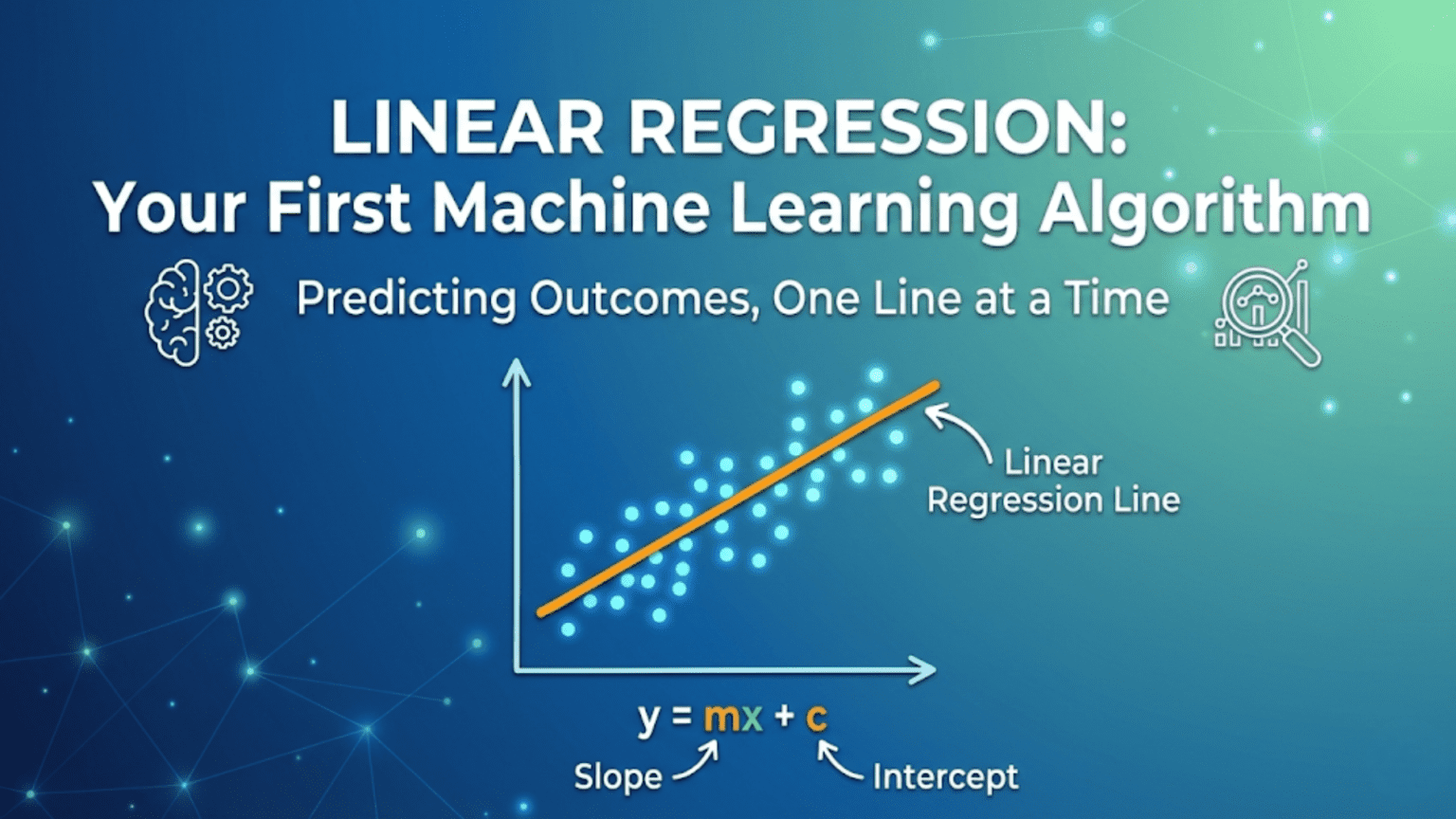
Linear regression is a supervised machine learning algorithm that models the relationship between a dependent variable (output) and one or more independent variables (inputs) by fitting a straight line through the data. It predicts continuous numerical outputs by learning a mathematical equation of the form ŷ = mx + b, where m is the slope (weight) and b is the intercept (bias). It is the simplest and most interpretable machine learning algorithm, and understanding it provides the foundation for more complex methods including neural networks and deep learning.
Introduction: The Algorithm That Started It All
Every journey into machine learning begins somewhere, and for most practitioners that somewhere is linear regression. Simple enough to understand completely in a single sitting, yet powerful enough to solve real problems in finance, healthcare, science, and business, linear regression is the perfect entry point into the world of machine learning.
The idea is beautifully straightforward: given data points, find the best straight line that describes the relationship between inputs and output. If you know the size of a house, can you predict its price? If you have a person’s years of experience, can you predict their salary? If you measure the temperature, can you predict ice cream sales? Linear regression answers all of these questions by learning a mathematical equation from historical data.
What makes linear regression especially valuable as a starting point is that it introduces every fundamental concept you’ll encounter throughout machine learning. Features, labels, parameters, the cost function, gradient descent, training, testing, predictions — all of these appear in linear regression in their simplest form. Master linear regression, and you have a conceptual framework that extends naturally to logistic regression, neural networks, and beyond.
This comprehensive guide walks through linear regression from the ground up. You’ll learn the intuition behind fitting a line to data, the mathematical formula, how the algorithm learns from data (cost function and gradient descent), evaluation metrics, assumptions, real-world applications, and complete Python implementations with scikit-learn and from scratch.
The Core Idea: Fitting a Line to Data
Linear regression learns to predict continuous numerical values by fitting a line (or hyperplane) to training data.
A Simple Example
Problem: Predict a person’s salary based on years of experience.
Training Data:
Years Experience    Salary ($)
1                   45,000
2                   50,000
3                   60,000
4                   65,000
5                   75,000
6                   80,000
7                   90,000
8                   95,000
9                   105,000
10 110,000Goal: Find the line that best represents this relationship so we can predict salary for new values.
Scatter Plot View:
Salary
$110k │                              ●
$100k │                         ●
$90k  │                    ●
$80k  │               ●
$70k  │          ●
$60k  │     ●
$50k  │  ●
$40k  │
      └──────────────────────────── Years
1 2 3 4 5 6 7 8 9 10Best-Fit Line:
Salary ≈ 7,500 × Years + 38,000

Example predictions:
3 years → $7,500×3 + $38,000 = $60,500
7 years → $7,500×7 + $38,000 = $90,500This line is what linear regression learns. It finds the equation that best captures the pattern in training data and uses it to predict new values.
What “Best Fit” Means
With data points scattered around, many possible lines exist. Linear regression finds the specific line that minimizes prediction error — the vertical distances between actual data points and the line.
Salary
      │            ↑ Error (point above line)
$90k  │       ●    |
      │    ────────┼──── Line
      │       |    ↓ Error (point below line)
$60k  │       ●
      └────────────────── Years

Best fit line = minimizes total squared errorsThe algorithm mathematically finds the line where the sum of squared errors is as small as possible — this is called the least squares solution.
The Mathematics: The Linear Equation
Simple Linear Regression (One Feature)
Equation:
ŷ = w × x + b

Where:
ŷ = predicted value (y-hat)
x = input feature
w = weight (slope)
b = bias (intercept)Interpretation:
- w (weight/slope): How much y changes for every 1-unit increase in x
- w = 7,500 means “each additional year of experience adds $7,500 to salary”
- b (bias/intercept): Predicted value when x = 0
- b = 38,000 means “starting salary with 0 experience is $38,000”
What the Algorithm Learns: The values of w and b that minimize prediction error on training data.
Multiple Linear Regression (Multiple Features)
When predicting from multiple inputs:
Equation:
ŷ = w₁x₁ + w₂x₂ + ... + wₙxₙ + b

Or in matrix form:
ŷ = Xw + b

Where:
x₁, x₂, ..., xₙ = input features
w₁, w₂, ..., wₙ = weights for each feature
b = biasExample: House Price Prediction
ŷ = w₁ × sqft + w₂ × bedrooms + w₃ × age + b

Learned weights:
w₁ = 150   (each sq ft adds $150)
w₂ = 8,000 (each bedroom adds $8,000)
w₃ = -500  (each year of age reduces price by $500)
b  = 50,000 (base price)

Prediction for 2,000 sqft, 3 bed, 10 years old:
ŷ = 150×2000 + 8000×3 + (-500)×10 + 50,000
  = 300,000 + 24,000 - 5,000 + 50,000
= $369,000How the Algorithm Learns: Cost Function and Optimization
Linear regression learns by minimizing a cost function — a measure of how wrong its predictions are.
The Cost Function: Mean Squared Error
MSE (Mean Squared Error):
J(w, b) = (1/m) × Σᵢ₌₁ᵐ (ŷᵢ - yᵢ)²

Where:
m = number of training examples
ŷᵢ = predicted value for example i
yᵢ = actual value for example i
(ŷᵢ - yᵢ) = error for example iWhy Squared Errors?
- Penalizes large errors more than small ones
- Makes the math clean (differentiable)
- Always positive (errors don’t cancel out)
- Convex function — guarantees single global minimum
Example Calculation:
Three training examples:
Actual:    y = [50, 70, 90]
Predicted: ŷ = [55, 65, 95]
Errors:        [5, -5, 5]
Squared:       [25, 25, 25]
MSE = (25 + 25 + 25) / 3 = 25

Goal: Find w and b that minimize this MSEThe Loss Landscape
With one weight w, the cost function J(w) is a bowl-shaped parabola:
Cost J(w)
    │     ╲       ╱
    │      ╲     ╱
    │       ╲   ╱
    │        ╲ ╱
    │         ✦  ← Minimum (best w)
└────────────── wLinear regression’s cost function is convex — it has exactly one global minimum. This means gradient descent will always find the optimal solution, unlike the jagged landscape of neural networks.
Learning: Gradient Descent
Process: Iteratively adjust w and b to reduce cost
Update Rules:
w = w - α × ∂J/∂w
b = b - α × ∂J/∂b

Where α = learning rate

Gradients:
∂J/∂w = (2/m) × Σᵢ₌₁ᵐ (ŷᵢ - yᵢ) × xᵢ
∂J/∂b = (2/m) × Σᵢ₌₁ᵐ (ŷᵢ - yᵢ)Iteration Example:
Initial: w=0, b=0, α=0.001

Training data: [(1,45), (2,50), (3,60)]

Iteration 1:
  Predictions: [0, 0, 0]
  Errors: [-45, -50, -60]
  ∂J/∂w = (2/3)[(-45×1) + (-50×2) + (-60×3)] = -116.67
  ∂J/∂b = (2/3)[(-45) + (-50) + (-60)] = -103.33

  Update:
  w = 0 - 0.001×(-116.67) = 0.117
  b = 0 - 0.001×(-103.33) = 0.103

Iteration 2: (repeat with new w, b)
  Better predictions → smaller errors → smaller gradients

Continue until convergence...Analytical Solution (Normal Equation)
Unlike neural networks, linear regression has a closed-form solution:
w = (XᵀX)⁻¹Xᵀy

Where:
X = feature matrix
y = target vectorAdvantages: Exact solution, no iterations, no learning rate to tune Disadvantages: Slow for very large datasets (matrix inversion is expensive)
scikit-learn uses this by default for small to medium datasets.
Step-by-Step: Complete Example
Let’s walk through a full linear regression workflow.
Dataset: Predicting Student Exam Scores
Data (hours studied vs. exam score):
Hours    Score
1.0      45
1.5      50
2.0      55
2.5      58
3.0      65
3.5      70
4.0      72
4.5      78
5.0      83
5.5      85
6.0      90
6.5      92
7.0 95Step 1: Explore the Data
import numpy as np
import pandas as pd
import matplotlib.pyplot as plt

# Data
hours  = np.array([1.0, 1.5, 2.0, 2.5, 3.0, 3.5, 4.0,
                   4.5, 5.0, 5.5, 6.0, 6.5, 7.0])
scores = np.array([45, 50, 55, 58, 65, 70, 72,
                   78, 83, 85, 90, 92, 95])

# Visualize
plt.scatter(hours, scores, color='blue', label='Actual')
plt.xlabel('Hours Studied')
plt.ylabel('Exam Score')
plt.title('Hours vs. Exam Score')
plt.legend()
plt.show()

# Basic stats
print(f"Correlation: {np.corrcoef(hours, scores)[0,1]:.3f}")
# Output: Correlation: 0.997 (very strong positive linear relationship)Step 2: Split Data
from sklearn.model_selection import train_test_split

X = hours.reshape(-1, 1)  # Must be 2D for scikit-learn
y = scores

X_train, X_test, y_train, y_test = train_test_split(
    X, y, test_size=0.2, random_state=42
)

print(f"Training: {len(X_train)} examples")
print(f"Testing: {len(X_test)} examples")
# Training: 10 examples
# Testing: 3 examplesStep 3: Train the Model
from sklearn.linear_model import LinearRegression

# Create and train model
model = LinearRegression()
model.fit(X_train, y_train)

# Learned parameters
print(f"Weight (slope): {model.coef_[0]:.2f}")
print(f"Bias (intercept): {model.intercept_:.2f}")
# Weight (slope): 7.84
# Bias (intercept): 38.21

# Equation: Score = 7.84 × Hours + 38.21
print(f"\nEquation: Score = {model.coef_[0]:.2f} × Hours + {model.intercept_:.2f}")Step 4: Make Predictions
# Predict on test set
y_pred = model.predict(X_test)

# Individual predictions
test_hours = np.array([[3.5], [5.5], [7.0]])
predictions = model.predict(test_hours)

for h, p in zip([3.5, 5.5, 7.0], predictions):
    print(f"Hours: {h} → Predicted Score: {p:.1f}")
# Hours: 3.5 → Predicted Score: 65.6
# Hours: 5.5 → Predicted Score: 81.3
# Hours: 7.0 → Predicted Score: 93.1

# New student: studied 4.2 hours
new_student = np.array([[4.2]])
prediction = model.predict(new_student)
print(f"\nNew student (4.2 hours): {prediction[0]:.1f}")
# New student (4.2 hours): 71.1Step 5: Evaluate the Model
from sklearn.metrics import mean_squared_error, mean_absolute_error, r2_score

# Predictions on test set
y_pred_test = model.predict(X_test)

# Metrics
mse  = mean_squared_error(y_test, y_pred_test)
rmse = np.sqrt(mse)
mae  = mean_absolute_error(y_test, y_pred_test)
r2   = r2_score(y_test, y_pred_test)

print(f"MSE:  {mse:.2f}")
print(f"RMSE: {rmse:.2f}")
print(f"MAE:  {mae:.2f}")
print(f"R²:   {r2:.4f}")
# MSE:  4.21
# RMSE: 2.05
# MAE:  1.72
# R²: 0.9944Step 6: Visualize the Fit
# Plot data and regression line
plt.figure(figsize=(8, 5))
plt.scatter(X_train, y_train, color='blue', label='Training data')
plt.scatter(X_test, y_test, color='green', label='Test data')

# Regression line
x_line = np.linspace(0.5, 8, 100).reshape(-1, 1)
y_line = model.predict(x_line)
plt.plot(x_line, y_line, color='red', label='Regression line')

plt.xlabel('Hours Studied')
plt.ylabel('Exam Score')
plt.title('Linear Regression: Hours vs. Score')
plt.legend()
plt.grid(True, alpha=0.3)
plt.show()Evaluating Linear Regression
Key Metrics
Mean Squared Error (MSE):
MSE = (1/m) Σ (yᵢ - ŷᵢ)²

Interpretation: Average squared error
Units: Squared units of target variable
Lower is betterRoot Mean Squared Error (RMSE):
RMSE = √MSE

Interpretation: Average error in same units as target
Example: RMSE=5 for salary prediction means average error ~$5
Lower is betterMean Absolute Error (MAE):
MAE = (1/m) Σ |yᵢ - ŷᵢ|

Interpretation: Average absolute error
Less sensitive to outliers than MSE/RMSE
Lower is betterR² Score (Coefficient of Determination):
R² = 1 - (SS_res / SS_tot)

SS_res = Σ(yᵢ - ŷᵢ)²  (residual sum of squares)
SS_tot = Σ(yᵢ - ȳ)²   (total sum of squares)

Interpretation:
- R² = 1.0: Perfect fit (model explains all variance)
- R² = 0.9: Model explains 90% of variance
- R² = 0.0: Model no better than predicting mean
- R² < 0.0: Model worse than predicting mean

Higher is better (max 1.0)Interpreting R²
R² = 0.95: Excellent — model explains 95% of variance
R² = 0.80: Good — explains 80%, some unexplained
R² = 0.50: Moderate — explains half the variance
R² = 0.20: Poor — mostly unexplained variance
R² = 0.00: No better than predicting the meanImportant: What counts as “good” R² depends on domain
- Physical sciences: 0.99+ expected
- Economics/social sciences: 0.50-0.80 acceptable
- Stock market prediction: 0.02 may be significant
Assumptions of Linear Regression
Linear regression works best when these assumptions hold:
1. Linearity
Assumption: Relationship between X and y is linear
Check: Plot X vs. y — does it look like a line?
Violation: Curved relationship
If data shows curve:
- Use polynomial regression
- Log-transform features
- Try non-linear models
2. Independence
Assumption: Training examples are independent of each other
Violation: Time series data (today’s value depends on yesterday’s)
Solution: Use time series models (ARIMA, LSTM)3. Homoscedasticity (Constant Variance)
Assumption: Residuals (errors) have constant variance across all X values
Check: Plot residuals vs. predicted values — should be random cloud
Violation: Errors grow larger for larger X values (fan shape)
Solution: Log-transform target variable4. Normality of Residuals
Assumption: Residuals approximately normally distributed
Check: Histogram of residuals, Q-Q plot
Impact: Affects statistical tests and confidence intervals
5. No Multicollinearity (for Multiple Regression)
Assumption: Features not highly correlated with each other
Violation: Two features measuring essentially same thing (height in cm and height in inches)
Check: Correlation matrix between features
Solution:
- Remove one of the correlated features
- Use PCA for dimensionality reduction
- Use regularization (Ridge, Lasso)Real-World Applications
Finance
- Stock price prediction: Predict future price from historical trends
- Credit scoring: Predict credit risk from financial features
- Revenue forecasting: Predict company revenue from growth metrics
Healthcare
- Drug dosage: Predict optimal drug dose from patient weight
- Medical cost prediction: Estimate costs from patient characteristics
- Disease progression: Track disease markers over time
Real Estate
- House price prediction: Predict prices from features (size, location, age)
- Rental rate estimation: Price apartments based on amenities
- Investment analysis: ROI prediction from property characteristics
Engineering and Science
- Quality control: Predict product quality from manufacturing parameters
- Energy consumption: Predict power usage from temperature, occupancy
- Material properties: Predict strength from composition
Marketing
- Sales forecasting: Predict sales from advertising spend
- Customer lifetime value: Estimate value from behavioral features
- Price elasticity: Understand price-demand relationship
From Scratch: Implementing Linear Regression
Building from scratch deepens understanding.
Gradient Descent Implementation
import numpy as np

class LinearRegressionScratch:
    def __init__(self, learning_rate=0.01, n_iterations=1000):
        self.lr = learning_rate
        self.n_iter = n_iterations
        self.w = None
        self.b = None
        self.loss_history = []

    def fit(self, X, y):
        m, n = X.shape  # m examples, n features
        self.w = np.zeros(n)
        self.b = 0

        for iteration in range(self.n_iter):
            # Forward pass: predictions
            y_pred = X @ self.w + self.b

            # Cost (MSE)
            cost = np.mean((y_pred - y) ** 2)
            self.loss_history.append(cost)

            # Gradients
            dw = (2/m) * (X.T @ (y_pred - y))
            db = (2/m) * np.sum(y_pred - y)

            # Update
            self.w -= self.lr * dw
            self.b -= self.lr * db

            if iteration % 100 == 0:
                print(f"Iteration {iteration}: Cost = {cost:.4f}")

    def predict(self, X):
        return X @ self.w + self.b

    def score(self, X, y):
        y_pred = self.predict(X)
        ss_res = np.sum((y - y_pred) ** 2)
        ss_tot = np.sum((y - np.mean(y)) ** 2)
        return 1 - (ss_res / ss_tot)

# Usage
X = hours.reshape(-1, 1)
y = scores

# Normalize features for gradient descent
X_norm = (X - X.mean()) / X.std()

model_scratch = LinearRegressionScratch(learning_rate=0.01, n_iterations=1000)
model_scratch.fit(X_norm, y)

print(f"\nR² on training data: {model_scratch.score(X_norm, y):.4f}")Normal Equation Implementation
class LinearRegressionNormal:
    def __init__(self):
        self.w = None
        self.b = None

    def fit(self, X, y):
        # Add bias column of ones
        X_b = np.column_stack([np.ones(len(X)), X])

        # Normal equation: θ = (XᵀX)⁻¹Xᵀy
        theta = np.linalg.inv(X_b.T @ X_b) @ X_b.T @ y

        self.b = theta[0]
        self.w = theta[1:]

    def predict(self, X):
        return X @ self.w + self.b

# Usage
model_normal = LinearRegressionNormal()
model_normal.fit(hours.reshape(-1, 1), scores)

print(f"Weight: {model_normal.w[0]:.4f}")
print(f"Bias: {model_normal.b:.4f}")Common Pitfalls and How to Avoid Them
Pitfall 1: Not Scaling Features
Problem: Features on very different scales cause gradient descent to converge slowly
# Problem example
X = [[0.1, 1000], [0.2, 2000]]  # Feature 2 is 10,000x larger
# Gradient descent struggles

# Solution: Standardize features
from sklearn.preprocessing import StandardScaler
scaler = StandardScaler()
X_scaled = scaler.fit_transform(X_train)Pitfall 2: Using Linear Regression for Non-Linear Data
Problem: Fitting a line to curved data gives poor results
Solution: Check scatter plots first; use polynomial regression or other models
Pitfall 3: Ignoring Outliers
Problem: Outliers disproportionately pull the regression line
Solution: Remove genuine outliers, use robust regression, or use MAE instead of MSE
Pitfall 4: Extrapolating Too Far
Problem: Linear regression predictions may be unreliable far outside training range
Training range: house sizes 500-3000 sqft
Prediction for: 10,000 sqft house
→ May be wildly wrong (model never saw examples this large)Pitfall 5: Confusing Correlation with Causation
Problem: Strong R² doesn’t mean X causes y
Ice cream sales correlate with drowning rates
→ Don't conclude ice cream causes drowning
→ Third variable (summer heat) explains bothComparison: Linear Regression vs. Other Methods
| Aspect | Linear Regression | Polynomial Regression | Decision Tree | Neural Network |
|---|---|---|---|---|
| Boundary | Linear only | Curved | Step-wise | Any shape |
| Interpretability | Very high | High | Medium | Low |
| Training speed | Very fast | Fast | Fast | Slow |
| Data needed | Small | Small-medium | Medium | Large |
| Overfitting risk | Low | Medium-High | High | High |
| Best for | Linear relationships | Gentle curves | Non-linear, categorical | Complex patterns |
Conclusion: The Foundation You’ll Return To
Linear regression is not just a beginner’s algorithm — it’s a foundation you’ll return to throughout your machine learning career. Its simplicity makes it the best baseline model: always try linear regression first, because if it works well, why use something more complex?
Understanding linear regression deeply provides the conceptual scaffolding for everything that follows:
The equation ŷ = wx + b reappears in every neuron of every neural network — just with more inputs and non-linear activations added.
The cost function (MSE) is the same loss used in regression networks, and understanding it helps interpret what training is doing.
Gradient descent — the same algorithm — trains both simple linear regression and GPT-4. The mechanics are identical; only the scale differs.
Overfitting, regularization, train/test splits — all introduced here, all apply everywhere.
When you encounter a new regression problem, linear regression is your starting point. If the relationship appears roughly linear, it may be all you need. When you build more complex models, linear regression serves as the sanity-check baseline. When you debug neural networks, linear regression intuition helps.
Master this algorithm — its math, its assumptions, its implementation, its strengths and weaknesses — and you’ve built the most important foundation in all of supervised machine learning.