Gradient descent is an iterative optimization algorithm that finds the minimum of a function by repeatedly taking steps in the direction of steepest descent (negative gradient). In machine learning, it minimizes the loss function by adjusting model parameters: computing the gradient of loss with respect to parameters, then updating parameters in the opposite direction of the gradient. The three main variants are batch gradient descent (using all training data per update), stochastic gradient descent (using one example per update), and mini-batch gradient descent (using small batches), each with different speed-accuracy tradeoffs.
Introduction: Finding the Bottom of the Hill
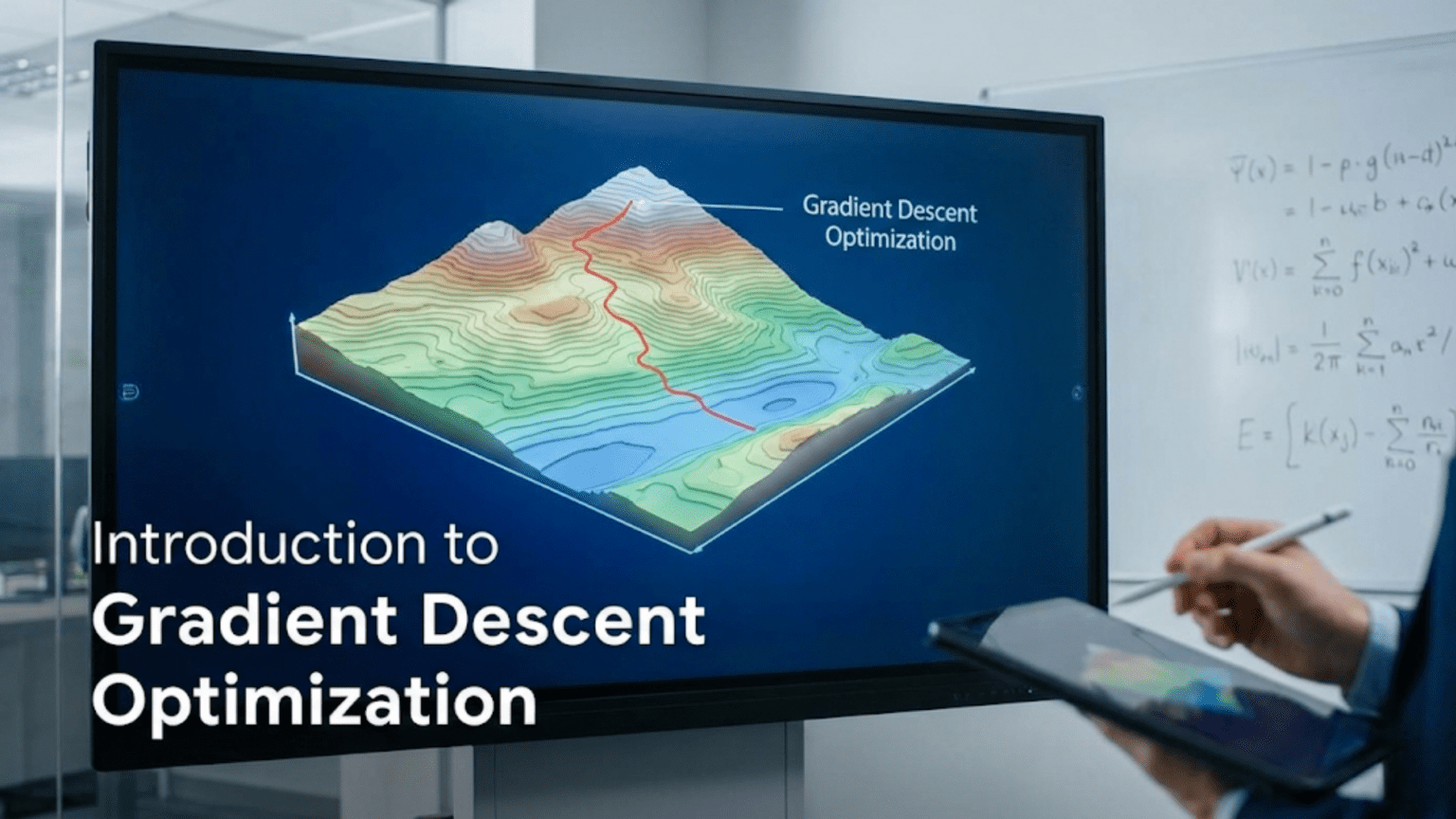
Imagine you’re hiking in dense fog at the top of a mountain. You can’t see where the valley is, but you want to descend to the lowest point. What do you do? You could feel the ground around you to determine which direction slopes downward most steeply, take a step in that direction, then repeat the process. Eventually, you’ll reach a valley—perhaps not the lowest point on the mountain, but at least a local low point.
This is exactly how gradient descent works. It’s a simple yet powerful algorithm for finding the minimum of a function when you can’t see the whole landscape. In machine learning, that function is the loss function, and the minimum represents the best model parameters—the weights and biases that make the most accurate predictions.
Gradient descent is the workhorse of machine learning optimization. Nearly every neural network you’ve heard of—from image classifiers to language models to game-playing agents—was trained using gradient descent or one of its variants. It’s the algorithm that turns backpropagation’s gradient calculations into actual learning, taking those gradients and using them to improve the model step by step.
Understanding gradient descent is essential for anyone working with machine learning. It determines how fast your model trains, whether it will converge to a good solution, and how to diagnose training problems. When you set a learning rate, choose between optimizers, or debug why a model won’t learn, you’re making decisions about how gradient descent operates.
This comprehensive guide introduces gradient descent from the ground up. You’ll learn the core algorithm, mathematical foundations, different variants (batch, stochastic, mini-batch), learning rate selection, advanced optimizers, common challenges and solutions, and practical implementation details.
The Optimization Problem
Before understanding gradient descent, let’s clarify what problem it solves.
The Goal: Minimize Loss
Given:
- Model with parameters θ (weights and biases)
- Loss function L(θ) measuring prediction error
- Training data to learn from
Goal: Find θ that minimizes L(θ)
Mathematical Statement:
θ* = argmin L(θ)
      θ

Find parameters θ* that give minimum lossWhy We Need Optimization
Can’t Solve Directly:
- Neural networks: Loss function too complex for analytical solution
- No formula like linear regression’s closed-form solution
- Must use iterative numerical methods
Example:
Linear Regression: Can solve directly
θ = (XᵀX)⁻¹Xᵀy  (closed-form solution)

Neural Network: No closed-form solution
Must use iterative optimization
The Loss Landscape
Visualizing Loss:
- Think of loss as landscape (hills and valleys)
- Height = loss value
- Position = parameter values
- Goal: Find lowest point (valley)
2D Example (one parameter):
Loss
 │     ╱‾╲
 │    ╱   ╲    ╱‾╲
 │   ╱     ╲  ╱   ╲
 │  ╱       ╲╱     ╲
 │─────────────────────θ
       ↑        ↑
     Local    Global
minimum minimumHigh Dimensions:
- Real networks: millions of parameters
- Can’t visualize
- Same principles apply
What is Gradient Descent?
Gradient descent is an iterative algorithm that finds the minimum by repeatedly moving in the direction of steepest descent.
The Core Idea
Step 1: Start at random point (initialize parameters)
Step 2: Calculate gradient (direction of steepest ascent)
∇L(θ) = gradient of loss with respect to parametersStep 3: Move opposite direction (downhill)
θ_new = θ_old - α × ∇L(θ)

Where α = learning rate (step size)Step 4: Repeat until convergence
The Gradient
Definition: Vector of partial derivatives
For parameter vector θ = [θ₁, θ₂, …, θₙ]:
∇L(θ) = [∂L/∂θ₁, ∂L/∂θ₂, ..., ∂L/∂θₙ]Properties:
- Points in direction of steepest increase
- Perpendicular to contour lines of L
- Magnitude indicates steepness
Why Negative Gradient:
- Gradient points uphill (increasing loss)
- Negative gradient points downhill (decreasing loss)
- We want to decrease loss → move in negative gradient direction
Visual Intuition
1D Example:
Loss
 │      ╱‾╲
 │     ╱   ╲
 │    ╱     ╲
 │   ╱       ╲
 │  •──→      ╲
 │─────────────────θ
    ↑
  Current position
Gradient positive → move left (decrease θ)2D Example (two parameters):
Contour plot of loss:

θ₂│        ╭─╮
  │      ╭───╮
  │    ╭─────╮
  │   ╭───•───╮  • = current position
  │  ╭─────────╮
  │ ╭───────────╮
  └─────────────────θ₁

Gradient points outward (away from minimum)
Negative gradient points inward (toward minimum)
Take step toward centerThe Algorithm: Step-by-Step
Batch Gradient Descent (BGD)
Uses: Entire training dataset for each update
Algorithm:
1. Initialize parameters θ randomly
2. Repeat until convergence:
   a. Compute gradient using ALL training data:
      ∇L(θ) = (1/m) Σᵢ₌₁ᵐ ∇L(θ; xⁱ, yⁱ)
      where m = number of training examples

   b. Update parameters:
      θ = θ - α × ∇L(θ)

c. Check convergence (e.g., gradient small enough)Pseudocode:
# Initialize
theta = random_initialization()
alpha = 0.01  # learning rate

# Repeat until convergence
for iteration in range(max_iterations):
    # Compute gradient on entire dataset
    gradient = compute_gradient(theta, X_train, y_train)

    # Update parameters
    theta = theta - alpha * gradient

    # Check convergence
    if convergence_criterion_met():
breakExample: Linear Regression
Problem: Fit line to data (y = mx + b)
Parameters: θ = [m, b]
Loss: Mean Squared Error
L(θ) = (1/2m) Σᵢ₌₁ᵐ (ŷⁱ - yⁱ)²
     = (1/2m) Σᵢ₌₁ᵐ (mxⁱ + b - yⁱ)²
Gradients:
∂L/∂m = (1/m) Σᵢ₌₁ᵐ (mxⁱ + b - yⁱ) × xⁱ
∂L/∂b = (1/m) Σᵢ₌₁ᵐ (mxⁱ + b - yⁱ)Update Rules:
m = m - α × ∂L/∂m
b = b - α × ∂L/∂bNumerical Example:
Data: (x, y) = [(1, 2), (2, 4), (3, 6)]
Initialization: m = 0, b = 0, α = 0.1
Iteration 1:
Predictions: ŷ = [0, 0, 0]
Errors: [−2, −4, −6]

∂L/∂m = (1/3)[(-2)(1) + (-4)(2) + (-6)(3)]
      = (1/3)[-2 - 8 - 18] = -28/3 = -9.33

∂L/∂b = (1/3)[-2 - 4 - 6] = -12/3 = -4

Updates:
m = 0 - 0.1 × (-9.33) = 0.933
b = 0 - 0.1 × (-4) = 0.4

New parameters: m=0.933, b=0.4Iteration 2:
Predictions: ŷ = [1.333, 2.266, 3.199]
Errors: [0.667, 1.734, 2.801]

∂L/∂m = (1/3)[(0.667)(1) + (1.734)(2) + (2.801)(3)]
      = (1/3)[11.47] = 3.82

∂L/∂b = (1/3)[5.20] = 1.73

Updates:
m = 0.933 - 0.1 × 3.82 = 0.551
b = 0.4 - 0.1 × 1.73 = 0.227

New parameters: m=0.551, b=0.227Continue until convergence…
Final Result: m ≈ 2, b ≈ 0 (true line: y = 2x)
Learning Rate: The Critical Hyperparameter
The learning rate α determines step size. Choosing it correctly is crucial.
Too Small Learning Rate
Problem: Convergence extremely slow
Visual:
Loss
 │      ╱‾╲
 │     ╱   ╲
 │    ╱     ╲
 │   •→•→•→•→╲
 │  ╱         ╲
 │─────────────────θ

Tiny steps → thousands of iterationsExample:
α = 0.00001
Takes 100,000 iterations to converge
Training time: hours instead of minutesToo Large Learning Rate
Problem: Overshooting, divergence, oscillation
Visual:
Loss
 │      ╱‾╲
 │     ╱   ╲
 │    ╱     ╲
 │   ╱    •  ╲
 │  •←──────→•╲
 │─────────────────θ

Oscillates, never settlesExample:
α = 10
Jumps over minimum
Loss increases instead of decreases
Training divergesJust Right Learning Rate
Sweet Spot: Converges quickly and smoothly
Visual:
Loss
 │      ╱‾╲
 │     ╱   ╲
 │    ╱  •  ╲
 │   ╱ •   • ╲
 │  •         ╲
 │─────────────────θ

Steady progress toward minimumTypical Values
Neural Networks: 0.001 - 0.1
Common starting point: 0.01

Linear Models: 0.01 - 1.0

Adjust based on:
- Loss behavior
- Gradient magnitudes
- Training stabilityLearning Rate Schedules
Fixed: Same α throughout training
Step Decay: Reduce α periodically
α = α₀ × 0.1^(epoch / drop_every)

Example: α = 0.1 initially, ×0.1 every 10 epochs
Epochs 0-9: α=0.1
Epochs 10-19: α=0.01
Epochs 20-29: α=0.001Exponential Decay:
α = α₀ × e^(-kt)1/t Decay:
α = α₀ / (1 + kt)Adaptive (Adam, RMSprop): Different α per parameter, automatically adjusted
Variants of Gradient Descent
Stochastic Gradient Descent (SGD)
Uses: Single random example per update
Algorithm:
1. Initialize θ
2. Repeat until convergence:
   For each example (xⁱ, yⁱ) in shuffled training data:
       a. Compute gradient on single example:
          ∇L(θ; xⁱ, yⁱ)

       b. Update:
θ = θ - α × ∇L(θ; xⁱ, yⁱ)Advantages:
- Much faster updates: m updates per epoch vs 1 (batch)
- Can escape local minima: Noise helps exploration
- Online learning: Update as data arrives
- Lower memory: Only need one example at a time
Disadvantages:
- Noisy updates: High variance in gradient estimates
- Doesn’t converge exactly: Oscillates around minimum
- Slower overall: Need more iterations to converge
When to Use:
- Very large datasets (millions of examples)
- Online learning scenarios
- When want fast initial progress
Mini-Batch Gradient Descent
Uses: Small batch of examples per update
Algorithm:
1. Initialize θ
2. Repeat until convergence:
   For each mini-batch B in shuffled training data:
       a. Compute gradient on batch:
          ∇L(θ) = (1/|B|) Σ_(x,y)∈B ∇L(θ; x, y)

       b. Update:
θ = θ - α × ∇L(θ)Batch Sizes: Typically 32, 64, 128, 256
Advantages:
- Balance: Speed of SGD + stability of batch GD
- Vectorization: Efficient matrix operations (GPU-friendly)
- Reduced variance: Smoother than SGD
- Practical: Works well in practice
Disadvantages:
- Hyperparameter: Must choose batch size
- Memory: Requires storing batch
When to Use:
- Default choice for deep learning
- Modern standard for neural networks
Comparison
| Aspect | Batch GD | Stochastic GD | Mini-Batch GD |
|---|---|---|---|
| Examples per update | All (m) | 1 | B (typically 32-256) |
| Updates per epoch | 1 | m | m/B |
| Convergence | Smooth, stable | Noisy, oscillates | Moderate noise |
| Speed per update | Slow | Very fast | Fast |
| Memory | High (all data) | Very low | Low-moderate |
| GPU utilization | Good | Poor | Excellent |
| Typical use | Small datasets | Rarely (too noisy) | Standard choice |
Advanced Optimizers
Basic gradient descent has limitations. Modern optimizers improve it.
Momentum
Problem: Gradient descent oscillates in ravines
Solution: Add velocity from previous steps
Algorithm:
v = β × v + (1 - β) × ∇L(θ)
θ = θ - α × v

Where:
- v = velocity
- β = momentum coefficient (typically 0.9)Effect:
- Accelerates in consistent directions
- Dampens oscillations
- Faster convergence
Visual:
Without momentum: •→←•→← (oscillates)
With momentum: •→→→→• (smooth)RMSprop (Root Mean Square Propagation)
Problem: Same learning rate for all parameters
Solution: Adaptive learning rate per parameter
Algorithm:
s = β × s + (1 - β) × (∇L(θ))²
θ = θ - α × ∇L(θ) / (√s + ε)

Where:
- s = moving average of squared gradients
- β ≈ 0.9
- ε = small constant (e.g., 10⁻⁸) for numerical stabilityEffect:
- Parameters with large gradients get smaller updates
- Parameters with small gradients get larger updates
- Adaptive per-parameter learning rates
Adam (Adaptive Moment Estimation)
Combines: Momentum + RMSprop
Algorithm:
m = β₁ × m + (1 - β₁) × ∇L(θ)      # First moment (momentum)
v = β₂ × v + (1 - β₂) × (∇L(θ))²  # Second moment (RMSprop)

m̂ = m / (1 - β₁ᵗ)  # Bias correction
v̂ = v / (1 - β₂ᵗ)

θ = θ - α × m̂ / (√v̂ + ε)

Default: β₁=0.9, β₂=0.999, ε=10⁻⁸Advantages:
- Generally works well “out of the box”
- Adaptive learning rates
- Handles sparse gradients well
- Most popular optimizer for deep learning
When to Use:
- Default choice for most deep learning
- Try first before others
AdaGrad
Idea: Adapt learning rate based on historical gradients
Good for: Sparse data, different feature frequencies
Limitation: Learning rate decays too aggressively
Comparison of Optimizers
| Optimizer | Advantages | Disadvantages | Best For |
|---|---|---|---|
| SGD | Simple, well-understood | Slow, needs tuning | Baselines, when have time to tune |
| SGD + Momentum | Faster, dampens oscillations | Still needs tuning | When SGD too slow |
| RMSprop | Adaptive rates, works well | Less common now | RNNs historically |
| Adam | Works well generally, adaptive | Can overfit on small data | Default choice |
| AdaGrad | Good for sparse data | Aggressive decay | NLP with rare words |
Implementation Examples
NumPy: Batch Gradient Descent
import numpy as np

def gradient_descent_batch(X, y, alpha=0.01, iterations=1000):
    """Batch gradient descent for linear regression"""
    m, n = X.shape  # m examples, n features
    theta = np.zeros(n)  # Initialize parameters
    loss_history = []

    for i in range(iterations):
        # Predictions
        predictions = X @ theta

        # Errors
        errors = predictions - y

        # Gradient (average over all examples)
        gradient = (1/m) * (X.T @ errors)

        # Update
        theta = theta - alpha * gradient

        # Track loss
        loss = (1/(2*m)) * np.sum(errors**2)
        loss_history.append(loss)

        # Print progress
        if i % 100 == 0:
            print(f"Iteration {i}, Loss: {loss:.4f}")

    return theta, loss_history

# Example usage
X = np.array([[1, 1], [1, 2], [1, 3]])  # Include bias term
y = np.array([2, 4, 6])

theta, history = gradient_descent_batch(X, y, alpha=0.1, iterations=1000)
print(f"Final parameters: {theta}")NumPy: Mini-Batch Gradient Descent
def gradient_descent_minibatch(X, y, alpha=0.01, epochs=100, batch_size=32):
    """Mini-batch gradient descent"""
    m, n = X.shape
    theta = np.zeros(n)

    for epoch in range(epochs):
        # Shuffle data
        indices = np.random.permutation(m)
        X_shuffled = X[indices]
        y_shuffled = y[indices]

        # Mini-batches
        for i in range(0, m, batch_size):
            # Get batch
            X_batch = X_shuffled[i:i+batch_size]
            y_batch = y_shuffled[i:i+batch_size]

            # Gradient on batch
            predictions = X_batch @ theta
            errors = predictions - y_batch
            gradient = (1/len(X_batch)) * (X_batch.T @ errors)

            # Update
            theta = theta - alpha * gradient

        # Epoch loss
        all_predictions = X @ theta
        loss = (1/(2*m)) * np.sum((all_predictions - y)**2)

        if epoch % 10 == 0:
            print(f"Epoch {epoch}, Loss: {loss:.4f}")

    return theta

theta = gradient_descent_minibatch(X, y, alpha=0.1, epochs=100, batch_size=2)TensorFlow/Keras: Using Optimizers
import tensorflow as tf
from tensorflow import keras

# Define model
model = keras.Sequential([
    keras.layers.Dense(64, activation='relu', input_shape=(10,)),
    keras.layers.Dense(32, activation='relu'),
    keras.layers.Dense(1)
])

# Different optimizers
sgd = keras.optimizers.SGD(learning_rate=0.01)
sgd_momentum = keras.optimizers.SGD(learning_rate=0.01, momentum=0.9)
rmsprop = keras.optimizers.RMSprop(learning_rate=0.001)
adam = keras.optimizers.Adam(learning_rate=0.001)

# Compile with optimizer
model.compile(optimizer=adam, loss='mse', metrics=['mae'])

# Train
model.fit(X_train, y_train, epochs=100, batch_size=32,
validation_data=(X_val, y_val))PyTorch: Custom Training Loop
import torch
import torch.nn as nn
import torch.optim as optim

# Model
model = nn.Sequential(
    nn.Linear(10, 64),
    nn.ReLU(),
    nn.Linear(64, 32),
    nn.ReLU(),
    nn.Linear(32, 1)
)

# Optimizer
optimizer = optim.Adam(model.parameters(), lr=0.001)

# Training loop
for epoch in range(100):
    for X_batch, y_batch in dataloader:
        # Forward pass
        predictions = model(X_batch)
        loss = nn.MSELoss()(predictions, y_batch)

        # Backward pass
        optimizer.zero_grad()  # Clear gradients
        loss.backward()         # Compute gradients
        optimizer.step()        # Update parameters

print(f"Epoch {epoch}, Loss: {loss.item():.4f}")Common Challenges and Solutions
Challenge 1: Slow Convergence
Symptoms: Loss decreases very slowly
Solutions:
- Increase learning rate (carefully)
- Use momentum or Adam
- Feature normalization (standardize inputs)
- Better initialization
- Check for bugs (gradient calculation)
Challenge 2: Oscillation/Divergence
Symptoms: Loss jumps around, increases
Solutions:
- Decrease learning rate
- Add gradient clipping
- Check data quality (outliers, errors)
- Use batch normalization
Challenge 3: Getting Stuck in Local Minima
Symptoms: Loss plateaus, not at global minimum
Solutions:
- Use momentum (helps escape)
- Try different initialization
- Add noise (SGD’s stochasticity helps)
- Increase model capacity (make landscape smoother)
Challenge 4: Vanishing/Exploding Gradients
Symptoms: Gradients become too small or too large
Solutions:
- Gradient clipping (cap maximum gradient)
- Proper initialization (Xavier, He)
- Batch normalization
- ReLU activation (vs sigmoid/tanh)
- Residual connections
Monitoring Gradient Descent
What to Track
1. Loss Curves:
plt.plot(train_loss, label='Training')
plt.plot(val_loss, label='Validation')
plt.xlabel('Epoch')
plt.ylabel('Loss')
plt.legend()Good: Both decreasing smoothly Bad: Training decreases, validation increases (overfitting)
2. Gradient Norms:
grad_norm = np.linalg.norm(gradients)
print(f"Gradient norm: {grad_norm}")Too small: Vanishing gradients Too large: Exploding gradients
3. Parameter Updates:
update_ratio = np.linalg.norm(updates) / np.linalg.norm(parameters)
print(f"Update ratio: {update_ratio}")Ideal: ~0.001 (updates about 0.1% of parameter values)
4. Learning Rate: Track if using schedule or adaptive methods
Practical Tips
1. Start with Adam
optimizer = Adam(learning_rate=0.001)Works well for most problems, good default choice.
2. Normalize Inputs
X = (X - X.mean(axis=0)) / X.std(axis=0)Helps gradient descent converge faster.
3. Use Mini-Batches
batch_size = 32 # or 64, 128, 256Good balance of speed and stability.
4. Monitor Training
Plot losses, check for:
- Steady decrease (good)
- Oscillation (reduce learning rate)
- Plateau (may need different architecture)
5. Learning Rate Finder
# Try range of learning rates
for lr in [1e-5, 1e-4, 1e-3, 1e-2, 1e-1]:
    test_optimizer(lr)

# Use one that decreases loss fastest without divergingConclusion: The Engine of Learning
Gradient descent is the optimization algorithm that powers machine learning. By iteratively computing gradients and taking steps in the direction that reduces loss, it enables models to learn from data—adjusting millions or billions of parameters to minimize prediction errors.
Understanding gradient descent means grasping:
The core principle: Follow the negative gradient (direction of steepest descent) to find lower loss, repeating until convergence.
The variants: Batch (stable but slow), stochastic (fast but noisy), mini-batch (practical balance).
The learning rate: The critical hyperparameter determining step size—too small and training is slow, too large and it diverges.
The modern optimizers: Momentum, RMSprop, and Adam that enhance basic gradient descent with adaptive learning rates and velocity.
The challenges: Local minima, saddle points, vanishing/exploding gradients, and how to address them.
Every time you train a machine learning model, gradient descent is working behind the scenes: computing gradients via backpropagation, updating parameters, gradually improving predictions. The loss curves you watch decrease during training show gradient descent in action, finding better and better parameter values.
As you build and train models, remember that choosing the right optimizer, setting appropriate learning rates, and monitoring gradient descent’s progress are critical for success. Adam works well as a default, but understanding the principles enables you to diagnose problems, tune hyperparameters effectively, and ultimately train better models.
Gradient descent might be conceptually simple—calculate gradient, take step, repeat—but this simple algorithm is what makes machine learning work, enabling the remarkable AI systems we see today.