Introduction: The Mathematical Engine of Machine Learning
Imagine teaching a child to throw a ball into a basket. After each throw, you give feedback: “throw a little harder” or “aim slightly to the left.” With each attempt, the child adjusts their technique based on your guidance, gradually improving until they consistently make the shot. This iterative process of making small adjustments to improve performance is remarkably similar to how machine learning algorithms learn, and at the heart of this learning process lies a fundamental mathematical concept: derivatives and gradients.
When you first encounter machine learning, you might wonder how a computer program can possibly “learn” from data. The answer lies in optimization, the process of finding the best possible solution to a problem. Machine learning models learn by repeatedly adjusting their internal parameters to minimize errors, and derivatives are the mathematical tools that tell the model exactly which direction to adjust and by how much. Without derivatives and gradients, modern machine learning as we know it simply wouldn’t exist.
In this comprehensive guide, we’ll explore the fascinating world of derivatives and gradients, building your understanding from the ground up. You’ll discover why these mathematical concepts are so crucial for artificial intelligence, how they power everything from simple linear regression to complex deep neural networks, and most importantly, how you can understand and use them in your own machine learning projects. Whether you’re completely new to calculus or need a refresher with a machine learning focus, this article will provide you with the foundational knowledge you need to understand the mathematics behind learning algorithms.
What Are Derivatives? Understanding the Rate of Change
Before we dive into how derivatives power machine learning, let’s first understand what a derivative actually is. At its core, a derivative measures how quickly something changes. Think of it as a mathematical speedometer that tells you the rate of change at any given moment.
Consider driving a car. If you look at your odometer, it tells you your position, showing you’ve traveled sixty miles. But if you want to know how fast you’re going right now, you look at the speedometer, which might show sixty miles per hour. The speedometer is showing you the rate of change of your position with respect to time, which is essentially a derivative. In mathematical terms, if your position is represented by a function, the derivative of that function gives you your velocity.
Let’s make this more concrete with a simple example. Suppose you have a function f(x) = x², which represents a parabola. When x equals two, the function value is four (since 2² = 4). But what if we want to know how steep the curve is at that point? How quickly is the function value changing as x changes? This is exactly what the derivative tells us.
The derivative of f(x) = x² is f'(x) = 2x. This derivative function tells us the slope of the original function at any point x. When x equals two, the derivative equals four (since 2 × 2 = 4), meaning that at x = 2, the function is increasing at a rate of four units vertically for every one unit horizontally. This slope information is crucial for machine learning because it tells us how changes in our inputs affect our outputs.
The Formal Definition of a Derivative
While we’ve been discussing derivatives intuitively, let’s look at the formal mathematical definition. The derivative of a function f(x) at a point x is defined as:
f'(x) = lim[h→0] (f(x + h) - f(x)) / hThis notation might look intimidating at first, but it’s actually expressing a beautifully simple idea. We’re looking at how much the function changes (the numerator) when we make a tiny change in x (the denominator), and we’re taking this to the limit as that change becomes infinitesimally small.
Let’s break this down step by step. The expression f(x + h) represents the function value at a point slightly to the right of x. The difference f(x + h) – f(x) tells us how much the function changed. We divide this change by h to get the average rate of change over that interval. As we let h approach zero, we’re zooming in on a single point, giving us the instantaneous rate of change, which is the derivative.
To see this in action, let’s calculate the derivative of f(x) = x² using this definition:
f'(x) = lim[h→0] ((x + h)² - x²) / h
      = lim[h→0] (x² + 2xh + h² - x²) / h
      = lim[h→0] (2xh + h²) / h
      = lim[h→0] (2x + h)
      = 2x
This confirms what we stated earlier: the derivative of x² is 2x. This process, while mathematically rigorous, can be tedious for complex functions, which is why we have derivative rules that make the process much faster.
Essential Derivative Rules for Machine Learning
In practice, you’ll rarely compute derivatives using the formal limit definition. Instead, you’ll use a set of rules that make finding derivatives quick and straightforward. Let’s explore the most important rules you’ll encounter in machine learning.
The Power Rule
The power rule is perhaps the most frequently used derivative rule. If you have a function of the form f(x) = x^n, where n is any real number, the derivative is:
f'(x) = n × x^(n-1)This rule is incredibly powerful in its simplicity. For example, if f(x) = x³, then f'(x) = 3x². If f(x) = x⁵, then f'(x) = 5x⁴. Even when n is negative or fractional, this rule still applies. For instance, if f(x) = 1/x = x^(-1), then f'(x) = -1 × x^(-2) = -1/x².
The power rule is fundamental in machine learning because polynomial functions and their variations appear constantly in our models. When we’re working with neural networks or regression models, we’re often dealing with weighted sums and polynomial transformations of our input features, all of which require the power rule for optimization.
The Constant Multiple Rule
If you multiply a function by a constant, you can factor that constant out when taking the derivative. Mathematically, if f(x) = c × g(x), where c is a constant, then:
f'(x) = c × g'(x)For example, if f(x) = 5x³, we can write this as 5 times x³. The derivative of x³ is 3x², so the derivative of 5x³ is simply 5 times 3x², which equals 15x². This rule is essential when dealing with weighted inputs in machine learning models, where each feature is multiplied by a learned weight parameter.
The Sum Rule
When you have a function that’s the sum of two or more functions, the derivative of the sum is simply the sum of the derivatives. If f(x) = g(x) + h(x), then:
f'(x) = g'(x) + h'(x)This rule is tremendously useful because machine learning models often involve complex expressions that are sums of many terms. For instance, if f(x) = x³ + 2x² – 5x + 7, we can take the derivative term by term: f'(x) = 3x² + 4x – 5. The constant term (7) disappears because the derivative of any constant is zero, which makes intuitive sense since constants don’t change.
The Chain Rule: Composing Functions
The chain rule is perhaps the most important derivative rule for machine learning, particularly for deep learning. It allows us to find the derivative of composite functions, which are functions within functions. If you have f(x) = g(h(x)), meaning you apply function h first and then apply function g to the result, the chain rule states:
f'(x) = g'(h(x)) × h'(x)Let’s work through a concrete example. Suppose f(x) = (x² + 1)³. We can think of this as an outer function g(u) = u³ applied to an inner function h(x) = x² + 1. Using the chain rule, we first take the derivative of the outer function with respect to its input: g'(u) = 3u². Then we multiply by the derivative of the inner function: h'(x) = 2x. Substituting back, we get:
f'(x) = 3(x² + 1)² × 2x = 6x(x² + 1)²The chain rule is absolutely fundamental to backpropagation, the algorithm that trains neural networks. Neural networks are essentially deeply nested composite functions, with each layer transforming the output of the previous layer. To train these networks, we need to compute how changes in the weights affect the final output, and the chain rule provides exactly the mechanism to propagate these changes backward through all the layers.
The Product Rule and Quotient Rule
When multiplying two functions together, we use the product rule. If f(x) = g(x) × h(x), then:
f'(x) = g'(x) × h(x) + g(x) × h'(x)For instance, if f(x) = x² × sin(x), then f'(x) = 2x × sin(x) + x² × cos(x).
When dividing functions, we use the quotient rule. If f(x) = g(x) / h(x), then:
f'(x) = (g'(x) × h(x) - g(x) × h'(x)) / (h(x))²While these rules appear less frequently in basic machine learning than the power rule or chain rule, they’re still important for understanding more complex model architectures and loss functions.
From Single Variables to Multiple Variables: Introducing Partial Derivatives
So far, we’ve focused on functions of a single variable, like f(x) = x². However, machine learning problems almost always involve multiple variables. A simple linear regression model predicting house prices might use features like square footage, number of bedrooms, and location. We need a way to understand how each of these variables independently affects our prediction.
This is where partial derivatives come in. A partial derivative measures how a function changes with respect to one specific variable while holding all other variables constant. Think of it like adjusting one knob on a sound mixing board while keeping all the other knobs fixed, then observing how the output changes.
Let’s consider a simple function of two variables: f(x, y) = x² + 3xy + y². This function takes two inputs and produces one output. We can take the partial derivative with respect to x, treating y as if it were a constant:
∂f/∂x = 2x + 3yThe symbol ∂ (pronounced “partial”) distinguishes partial derivatives from ordinary derivatives. Notice that when we differentiated with respect to x, the term y² disappeared because it’s treated as a constant (and the derivative of a constant is zero), while the term 3xy became 3y because y is held constant.
Similarly, we can take the partial derivative with respect to y:
∂f/∂y = 3x + 2yThese partial derivatives tell us important information. The partial derivative ∂f/∂x tells us how much f changes when we make a small change to x while keeping y fixed. The partial derivative ∂f/∂y tells us how much f changes when we make a small change to y while keeping x fixed.
In machine learning, we’re constantly working with functions that depend on many variables. A neural network might have millions of parameters, and we need to compute partial derivatives with respect to each one. These partial derivatives tell us how to adjust each parameter to improve the model’s performance.
Understanding Gradients: Vectors of Change
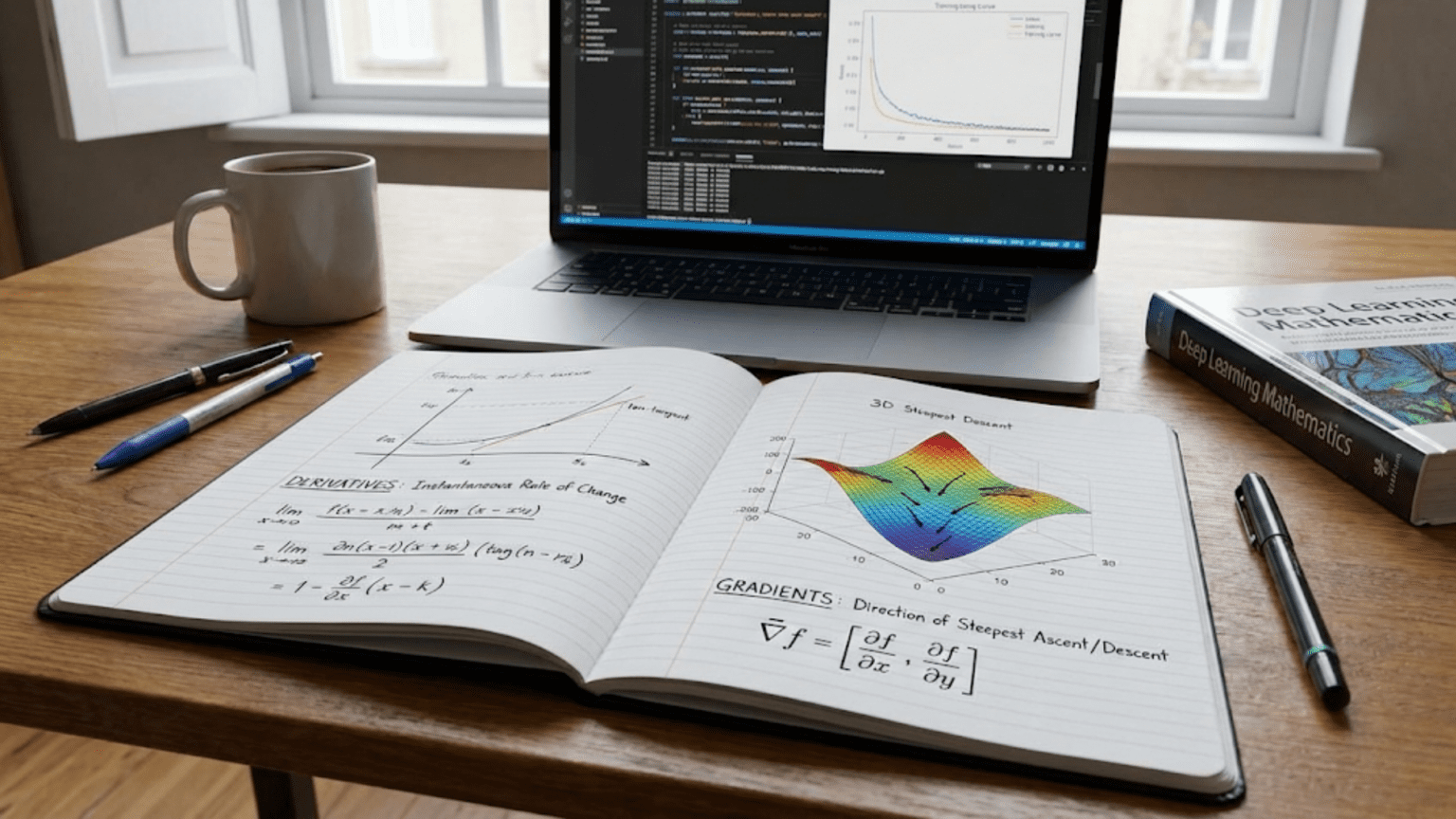
Now we arrive at one of the most crucial concepts in machine learning: the gradient. The gradient is simply a vector that contains all the partial derivatives of a function. It points in the direction of steepest increase of the function and tells us how steeply the function is changing in that direction.
For our function f(x, y) = x² + 3xy + y², the gradient is:
∇f = [∂f/∂x, ∂f/∂y] = [2x + 3y, 3x + 2y]The symbol ∇ (pronounced “nabla” or “del”) represents the gradient operator. The gradient is a vector with as many components as there are input variables. For a function of three variables, the gradient would have three components, and so on.
Let’s evaluate this gradient at a specific point to make it more concrete. At the point (x=1, y=2), we have:
∇f(1, 2) = [2(1) + 3(2), 3(1) + 2(2)] = [8, 7]This gradient vector [8, 7] tells us that at the point (1, 2), the function is increasing most rapidly in the direction of this vector. If we want to maximize the function, we should move in this direction. Conversely, if we want to minimize the function (which is usually what we want in machine learning), we should move in the opposite direction: [-8, -7].
The magnitude of the gradient vector tells us how steep the function is. A large magnitude means the function is changing rapidly, while a small magnitude means the function is relatively flat. When the gradient is zero, we’re at a stationary point, which could be a minimum, maximum, or saddle point.
Visualizing Gradients in Two Dimensions
Imagine you’re standing on a hillside, and you want to find the path that descends most quickly. At each point where you’re standing, the gradient vector points in the direction of steepest ascent up the hill. The negative gradient (pointing in the opposite direction) shows the path of steepest descent.
In machine learning, we’re usually trying to minimize some error or loss function. The landscape of this function might be incredibly complex with many hills and valleys, but the gradient always tells us the local direction of steepest descent. By repeatedly taking small steps in the direction of the negative gradient, we can navigate this complex landscape and find low points (minima) where our model performs well.
Gradient Descent: The Learning Algorithm
Now that we understand derivatives and gradients, we can appreciate how machine learning models actually learn. The fundamental algorithm underlying most machine learning is called gradient descent, and it’s a beautifully simple idea built entirely on the concepts we’ve been discussing.
Gradient descent is an iterative optimization algorithm that finds the minimum of a function by repeatedly moving in the direction of the negative gradient. The algorithm follows these steps:
- Start with initial parameter values (often random).
- Calculate the gradient of the loss function with respect to the parameters.
- Update the parameters by moving a small step in the direction opposite to the gradient.
- Repeat steps two and three until the algorithm converges (the gradient becomes very small or we reach a maximum number of iterations).
Let’s express this mathematically. If θ represents our parameters and L(θ) represents our loss function (a measure of how poorly our model is performing), the gradient descent update rule is:
θ_new = θ_old - α × ∇L(θ_old)Here, α (alpha) is called the learning rate, a hyperparameter that controls how large each step is. The negative sign ensures we’re moving in the direction of decreasing loss (downhill rather than uphill).
A Simple Example: Finding the Minimum of a Function
Let’s work through a complete example to see gradient descent in action. Suppose we want to find the minimum of the function f(x) = x² – 4x + 4, which is a simple parabola.
First, we calculate the derivative: f'(x) = 2x – 4.
Let’s start with an initial guess of x = 0 and use a learning rate of α = 0.1. Here’s how the first few iterations proceed:
Iteration 1:
- Current position: x = 0
- Gradient: f'(0) = 2(0) – 4 = -4
- Update: x = 0 – 0.1 × (-4) = 0.4
Iteration 2:
- Current position: x = 0.4
- Gradient: f'(0.4) = 2(0.4) – 4 = -3.2
- Update: x = 0.4 – 0.1 × (-3.2) = 0.72
Iteration 3:
- Current position: x = 0.72
- Gradient: f'(0.72) = 2(0.72) – 4 = -2.56
- Update: x = 0.72 – 0.1 × (-2.56) = 0.976
We can see that with each iteration, we’re getting closer to x = 2, which is the true minimum of this function (you can verify this by setting the derivative equal to zero: 2x – 4 = 0, giving x = 2).
Implementing Gradient Descent in Python
Let’s implement this simple gradient descent example in Python to make it more concrete:
import numpy as np
import matplotlib.pyplot as plt

<em># Define the function and its derivative</em>
def f(x):
    """Our objective function: f(x) = x² - 4x + 4"""
    return x**2 - 4*x + 4

def gradient(x):
    """Derivative of f: f'(x) = 2x - 4"""
    return 2*x - 4

<em># Gradient descent parameters</em>
learning_rate = 0.1
initial_x = 0.0
num_iterations = 20

<em># Store the path for visualization</em>
x_history = [initial_x]
f_history = [f(initial_x)]

<em># Run gradient descent</em>
x = initial_x
for i in range(num_iterations):
    <em># Calculate the gradient at current position</em>
    grad = gradient(x)

    <em># Update x by moving in the opposite direction of the gradient</em>
    x = x - learning_rate * grad

    <em># Store the history</em>
    x_history.append(x)
    f_history.append(f(x))

    <em># Print progress</em>
    print(f"Iteration {i+1}: x = {x:.4f}, f(x) = {f(x):.4f}, gradient = {grad:.4f}")

print(f"\nFinal result: x = {x:.4f}, f(x) = {f(x):.4f}")
print(f"True minimum: x = 2.0, f(x) = 0.0")

<em># Visualize the optimization process</em>
x_range = np.linspace(-1, 4, 100)
y_range = f(x_range)

plt.figure(figsize=(10, 6))
plt.plot(x_range, y_range, 'b-', linewidth=2, label='f(x) = x² - 4x + 4')
plt.plot(x_history, f_history, 'ro-', markersize=8, label='Gradient Descent Path')
plt.xlabel('x')
plt.ylabel('f(x)')
plt.title('Gradient Descent Optimization')
plt.legend()
plt.grid(True)
plt.show()This code demonstrates several important aspects of gradient descent. First, notice how we iteratively update our position based on the gradient. Second, observe that the steps get smaller as we approach the minimum because the gradient itself becomes smaller near the minimum. This is actually a helpful property because it means we naturally slow down as we get close to our target, reducing the risk of overshooting.
The Learning Rate: Finding the Right Step Size
The learning rate α is one of the most important hyperparameters in gradient descent. It controls how big each step is in the direction of the negative gradient. Choosing the right learning rate is crucial for successful optimization.
If the learning rate is too small, the algorithm will eventually reach the minimum, but it will take a very long time to get there. Imagine trying to descend a mountain by taking tiny baby steps. You’ll eventually reach the bottom, but it might take days instead of hours.
On the other hand, if the learning rate is too large, the algorithm might overshoot the minimum and potentially even diverge, bouncing around wildly and never settling down. Picture trying to walk down a steep hillside while taking giant leaps. You might jump right over the valley floor and land on the opposite hillside, then jump back, repeatedly overshooting your target.
Let’s see this in action with our previous example. If we use a learning rate of 1.5 (much larger than our earlier 0.1), here’s what happens:
<em># Using a learning rate that's too large</em>
learning_rate_large = 1.5
x = 0.0

for i in range(10):
    grad = gradient(x)
    x = x - learning_rate_large * grad
print(f"Iteration {i+1}: x = {x:.4f}, f(x) = {f(x):.4f}")You’ll notice that the values oscillate wildly and don’t converge to the minimum. This is a clear sign that the learning rate is too large.
In practice, finding the right learning rate often involves experimentation. Common approaches include:
- Learning rate schedules: Start with a larger learning rate and gradually decrease it over time. This allows for fast initial progress while ensuring convergence later.
- Adaptive learning rates: Algorithms like Adam, RMSprop, and AdaGrad automatically adjust the learning rate for each parameter based on the history of gradients.
- Learning rate finder: Run the algorithm with exponentially increasing learning rates and plot the loss to find the optimal range.
Multivariable Gradient Descent: The Real Machine Learning Case
In real machine learning applications, we’re almost never optimizing a function of just one variable. Instead, we typically have hundreds, thousands, or even millions of parameters. The beautiful thing is that gradient descent scales naturally to these high-dimensional spaces.
Consider a simple linear regression problem where we’re trying to predict house prices. We might have a model like:
price = w₁ × square_feet + w₂ × bedrooms + w₃ × bathrooms + bHere we have four parameters: three weights (w₁, w₂, w₃) and one bias term (b). Our loss function measures how far off our predictions are from the actual prices, typically using mean squared error:
L(w₁, w₂, w₃, b) = (1/n) × Σ(predicted_price - actual_price)²To perform gradient descent, we need the partial derivative of the loss with respect to each parameter. The gradient is:
∇L = [∂L/∂w₁, ∂L/∂w₂, ∂L/∂w₃, ∂L/∂b]Each component tells us how to adjust the corresponding parameter. The update rule becomes:
w₁_new = w₁_old - α × ∂L/∂w₁
w₂_new = w₂_old - α × ∂L/∂w₂
w₃_new = w₃_old - α × ∂L/∂w₃
b_new = b_old - α × ∂L/∂b
Let’s implement a complete linear regression example using gradient descent:
import numpy as np

<em># Generate synthetic data</em>
np.random.seed(42)
n_samples = 100
X = np.random.randn(n_samples, 2)  <em># Two features</em>
true_weights = np.array([3.0, -2.0])
true_bias = 1.0
y = X.dot(true_weights) + true_bias + np.random.randn(n_samples) * 0.5

<em># Initialize parameters</em>
weights = np.zeros(2)
bias = 0.0
learning_rate = 0.01
num_iterations = 1000

<em># Gradient descent</em>
for iteration in range(num_iterations):
    <em># Forward pass: compute predictions</em>
    predictions = X.dot(weights) + bias

    <em># Compute error</em>
    error = predictions - y

    <em># Compute gradients</em>
    gradient_weights = (2/n_samples) * X.T.dot(error)
    gradient_bias = (2/n_samples) * np.sum(error)

    <em># Update parameters</em>
    weights = weights - learning_rate * gradient_weights
    bias = bias - learning_rate * gradient_bias

    <em># Compute and print loss every 100 iterations</em>
    if iteration % 100 == 0:
        loss = np.mean(error**2)
        print(f"Iteration {iteration}: Loss = {loss:.4f}")

print(f"\nFinal weights: {weights}")
print(f"True weights: {true_weights}")
print(f"Final bias: {bias:.4f}")
print(f"True bias: {true_bias:.4f}")This code demonstrates all the key concepts we’ve discussed: computing predictions, calculating errors, computing gradients for multiple parameters, and updating those parameters iteratively.
Backpropagation: Gradients in Neural Networks
Neural networks represent the most sophisticated application of derivatives and gradients in machine learning. A neural network is essentially a complex composite function with many layers, and training it requires computing gradients with respect to potentially millions of parameters.
The backpropagation algorithm is how we efficiently compute these gradients. It’s a direct application of the chain rule, propagating the error backward through the network layer by layer.
Consider a simple neural network with one hidden layer:
Input → Hidden Layer → Output Layer → LossMathematically, this looks like:
h = σ(W₁x + b₁)  # Hidden layer with activation σ
y = W₂h + b₂     # Output layer
L = (y - target)² # Loss function
To train this network, we need to compute ∂L/∂W₁, ∂L/∂b₁, ∂L/∂W₂, and ∂L/∂b₂. The backpropagation algorithm computes these efficiently using the chain rule.
Let’s work through the derivatives step by step:
For the output layer weights W₂:
∂L/∂W₂ = ∂L/∂y × ∂y/∂W₂The first term ∂L/∂y is straightforward since L = (y – target)²:
∂L/∂y = 2(y - target)The second term ∂y/∂W₂ is also simple since y = W₂h + b₂:
∂y/∂W₂ = hTherefore:
∂L/∂W₂ = 2(y - target) × hFor the hidden layer weights W₁: This requires more chain rule applications:
∂L/∂W₁ = ∂L/∂y × ∂y/∂h × ∂h/∂W₁We already know ∂L/∂y. The term ∂y/∂h equals W₂ (since y = W₂h + b₂). The term ∂h/∂W₁ involves the derivative of the activation function σ.
This demonstrates why backpropagation is so named: we start with the loss at the end and propagate the gradients backward through each layer, using the chain rule at each step.
Here’s a simple implementation of backpropagation for a two-layer network:
import numpy as np

def sigmoid(x):
    """Sigmoid activation function"""
    return 1 / (1 + np.exp(-x))

def sigmoid_derivative(x):
    """Derivative of sigmoid function"""
    s = sigmoid(x)
    return s * (1 - s)

<em># Network architecture</em>
input_size = 2
hidden_size = 3
output_size = 1

<em># Initialize weights randomly</em>
np.random.seed(42)
W1 = np.random.randn(input_size, hidden_size) * 0.1
b1 = np.zeros(hidden_size)
W2 = np.random.randn(hidden_size, output_size) * 0.1
b2 = np.zeros(output_size)

<em># Training data (XOR problem)</em>
X = np.array([[0, 0], [0, 1], [1, 0], [1, 1]])
y = np.array([[0], [1], [1], [0]])

learning_rate = 0.5
num_epochs = 10000

<em># Training loop</em>
for epoch in range(num_epochs):
    <em># Forward pass</em>
    z1 = X.dot(W1) + b1  <em># Hidden layer pre-activation</em>
    a1 = sigmoid(z1)      <em># Hidden layer activation</em>
    z2 = a1.dot(W2) + b2  <em># Output layer pre-activation</em>
    a2 = sigmoid(z2)      <em># Output layer activation (predictions)</em>

    <em># Compute loss</em>
    loss = np.mean((a2 - y) ** 2)

    <em># Backward pass</em>
    <em># Output layer gradients</em>
    dL_da2 = 2 * (a2 - y) / len(X)  <em># Loss gradient</em>
    da2_dz2 = sigmoid_derivative(z2)  <em># Activation gradient</em>
    dz2 = dL_da2 * da2_dz2  <em># Combine using chain rule</em>

    dW2 = a1.T.dot(dz2)  <em># Gradient for W2</em>
    db2 = np.sum(dz2, axis=0)  <em># Gradient for b2</em>

    <em># Hidden layer gradients</em>
    da1 = dz2.dot(W2.T)  <em># Propagate error back</em>
    da1_dz1 = sigmoid_derivative(z1)  <em># Activation gradient</em>
    dz1 = da1 * da1_dz1  <em># Combine using chain rule</em>

    dW1 = X.T.dot(dz1)  <em># Gradient for W1</em>
    db1 = np.sum(dz1, axis=0)  <em># Gradient for b1</em>

    <em># Update weights</em>
    W1 -= learning_rate * dW1
    b1 -= learning_rate * db1
    W2 -= learning_rate * dW2
    b2 -= learning_rate * db2

    <em># Print progress</em>
    if epoch % 1000 == 0:
        print(f"Epoch {epoch}: Loss = {loss:.6f}")

<em># Test the trained network</em>
print("\nFinal predictions:")
final_predictions = sigmoid(sigmoid(X.dot(W1) + b1).dot(W2) + b2)
for i in range(len(X)):
    print(f"Input: {X[i]}, Target: {y[i][0]}, Prediction: {final_predictions[i][0]:.4f}")
This implementation shows how the chain rule is applied at each layer to compute gradients, and how those gradients are used to update the weights. The beauty of backpropagation is that it efficiently computes all necessary gradients in a single backward pass through the network.
Common Activation Functions and Their Derivatives
In neural networks, activation functions introduce nonlinearity, allowing networks to learn complex patterns. Understanding these functions and their derivatives is crucial because we need these derivatives during backpropagation.
Sigmoid Function
The sigmoid function is defined as:
σ(x) = 1 / (1 + e^(-x))It squashes any input value to the range (0, 1), making it useful for binary classification. Its derivative has a particularly elegant form:
σ'(x) = σ(x) × (1 - σ(x))This means we can compute the derivative using just the function value itself, which is computationally efficient during backpropagation.
Hyperbolic Tangent (tanh)
The tanh function is defined as:
tanh(x) = (e^x - e^(-x)) / (e^x + e^(-x))It squashes inputs to the range (-1, 1) and is zero-centered, which can make optimization easier. Its derivative is:
tanh'(x) = 1 - tanh²(x)Rectified Linear Unit (ReLU)
ReLU has become the most popular activation function in deep learning. It’s defined as:
ReLU(x) = max(0, x)Its derivative is wonderfully simple:
ReLU'(x) = 1 if x > 0, else 0This simplicity makes ReLU computationally efficient and helps prevent the vanishing gradient problem that plagued earlier deep networks.
Leaky ReLU
To address the “dying ReLU” problem where neurons can get stuck outputting zero, Leaky ReLU allows a small negative slope:
Leaky ReLU(x) = max(0.01x, x)Its derivative is:
Leaky ReLU'(x) = 1 if x > 0, else 0.01The Vanishing and Exploding Gradient Problems
As neural networks become deeper, computing gradients through many layers can lead to problems. These issues arise directly from how the chain rule multiplies gradients together during backpropagation.
Vanishing Gradients
When we backpropagate through many layers, we multiply many gradient terms together. If these terms are small (less than one), multiplying many of them results in an exponentially smaller number. This is the vanishing gradient problem.
Consider a network with ten layers where each layer’s gradient is 0.5. The gradient for the first layer would be approximately:
0.5^10 = 0.00098This tiny gradient means the early layers learn extremely slowly or not at all. The sigmoid and tanh activation functions are particularly prone to this because their derivatives are always less than one.
Exploding Gradients
Conversely, if gradients are large (greater than one), multiplying them together can lead to exponentially large values. This is the exploding gradient problem, which can cause numerical instability and make training impossible.
Modern solutions to these problems include:
- Careful weight initialization: Methods like Xavier or He initialization ensure weights start in a range that prevents extreme gradient values.
- ReLU activation: The derivative of ReLU is exactly one for positive inputs, preventing multiplicative shrinking.
- Batch normalization: Normalizes layer inputs to maintain consistent gradient magnitudes.
- Gradient clipping: Limits gradient values to a maximum threshold to prevent explosion.
- Residual connections: Skip connections allow gradients to flow directly through the network.
Higher-Order Derivatives: Beyond the First Derivative
While first derivatives (gradients) are essential for optimization, second derivatives provide additional useful information. The second derivative tells us about the curvature of a function, which can help us choose better step sizes and understand the optimization landscape better.
The Hessian matrix contains all second-order partial derivatives of a function. For a function f(x, y), the Hessian is:
H = [∂²f/∂x²    ∂²f/∂x∂y]
    [∂²f/∂y∂x   ∂²f/∂y² ]
Second-order optimization methods use the Hessian to take more informed steps toward the minimum. However, computing and storing the Hessian becomes prohibitively expensive for the high-dimensional problems typical in machine learning.
Newton’s method is a classic second-order optimization algorithm that uses the update rule:
θ_new = θ_old - H^(-1) × ∇fWhile more accurate per iteration than gradient descent, the computational cost makes it impractical for large neural networks. However, the insights from second-order methods have inspired quasi-Newton methods and optimizers like L-BFGS that approximate second-order information more efficiently.
Automatic Differentiation: How Modern Deep Learning Frameworks Compute Gradients
In practice, you rarely compute gradients by hand. Modern deep learning frameworks like TensorFlow, PyTorch, and JAX use automatic differentiation to compute gradients automatically. This is neither symbolic differentiation (like what a computer algebra system would do) nor numerical differentiation (approximating with finite differences), but something more elegant and efficient.
Automatic differentiation works by breaking down complex functions into elementary operations (addition, multiplication, exponentials, etc.) and applying the chain rule systematically. Modern frameworks build a computational graph that tracks all operations, then traverse this graph backward to compute gradients efficiently.
Here’s a simple example using PyTorch:
import torch

<em># Define variables that require gradients</em>
x = torch.tensor(2.0, requires_grad=True)
y = torch.tensor(3.0, requires_grad=True)

<em># Define a function</em>
z = x**2 + 3*x*y + y**2

<em># Compute gradients automatically</em>
z.backward()

<em># Access the computed gradients</em>
print(f"∂z/∂x = {x.grad}")  <em># Should be 2x + 3y = 2(2) + 3(3) = 13</em>
print(f"∂z/∂y = {y.grad}") <em># Should be 3x + 2y = 3(2) + 2(3) = 12</em>This automatic differentiation is what makes modern deep learning possible. Without it, computing gradients for networks with millions of parameters would be practically impossible.
Practical Tips for Working with Gradients
As you work with machine learning models, here are some practical considerations related to gradients:
Checking Your Gradients
When implementing complex models or custom layers, it’s wise to verify your gradient calculations using numerical gradient checking. The idea is to approximate the gradient using the definition:
def numerical_gradient(f, x, epsilon=1e-5):
    """
    Compute numerical gradient approximation
    f: function to differentiate
    x: point at which to compute gradient
    epsilon: small perturbation
    """
return (f(x + epsilon) - f(x - epsilon)) / (2 * epsilon)Compare this numerical approximation to your analytical gradient. If they match (within reasonable tolerance), your gradient computation is likely correct.
Gradient Clipping
To prevent exploding gradients, especially in recurrent neural networks, gradient clipping limits gradient magnitudes:
<em># Clip gradients to maximum norm</em>
max_norm = 1.0
torch.nn.utils.clip_grad_norm_(model.parameters(), max_norm)Monitoring Gradients During Training
Watch for these warning signs:
- Gradients near zero: Indicates vanishing gradients or dead neurons
- Gradients exploding to infinity: Suggests your learning rate is too high or you need gradient clipping
- Oscillating loss: Often means the learning rate is too large
Most deep learning frameworks provide tools to visualize gradient distributions during training, which can help diagnose problems early.
Conclusion: The Foundation of Learning
Derivatives and gradients are truly the mathematical engine that powers machine learning. From simple linear regression to complex deep neural networks, the ability to compute how changes in parameters affect our objectives is what enables models to learn.
We’ve journeyed from the basic concept of a derivative as a rate of change, through the mechanics of gradient descent, to the sophisticated backpropagation algorithm that trains modern neural networks. Along the way, we’ve seen how the chain rule enables us to propagate errors backward through nested functions, how different activation functions affect gradient flow, and how automatic differentiation makes all of this practical at scale.
The beauty of these mathematical tools is that they provide a systematic, principled way to optimize incredibly complex functions with millions of parameters. Every time a neural network learns to recognize images, translate languages, or play games at superhuman levels, it’s fundamentally using derivatives and gradients to navigate the landscape of possible solutions.
As you continue your machine learning journey, you’ll encounter many variations and extensions of these core ideas: momentum-based optimizers that smooth out gradient updates, adaptive learning rate methods that automatically adjust step sizes, second-order methods that use curvature information, and advanced architectures that carefully manage gradient flow. But all of these build on the fundamental concepts we’ve explored here.
Understanding derivatives and gradients doesn’t just help you use machine learning tools more effectively; it gives you insight into why certain design choices work, how to diagnose and fix training problems, and how to develop new techniques. Whether you’re debugging a model that won’t converge, designing a custom architecture, or reading the latest research papers, a solid grasp of these mathematical foundations will serve you well.
The remarkable thing is that these powerful tools, which enable computers to learn from data and improve through experience, are built on relatively simple mathematical principles. A derivative is just a rate of change. A gradient is just a collection of derivatives. Gradient descent is just repeatedly taking small steps downhill. Yet from these simple building blocks emerge the sophisticated learning systems transforming our world.
As you move forward in your machine learning studies, keep coming back to these fundamentals. When you encounter a new optimization algorithm, think about how it’s modifying the basic gradient descent idea. When you see a new network architecture, consider how it affects gradient flow during backpropagation. The concepts of derivatives and gradients will remain central to understanding how machines learn, no matter how advanced the techniques become.