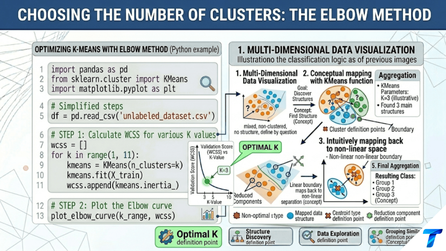
The elbow method plots within-cluster sum of squares (inertia) against the number of clusters k. As k increases, inertia always decreases — but with diminishing returns. The “elbow” is the point where adding another cluster provides little additional reduction in inertia, suggesting that the data naturally contains that many groups. Because the elbow is often ambiguous, use it alongside the silhouette score (which has a clear maximum) and the gap statistic (which compares inertia to a reference random distribution) for a more reliable choice.
Introduction
Every K-Means application forces the same decision: choose k. The algorithm will produce k clusters regardless of what k is — it will find three groups in data that naturally has five, or five groups in data that naturally has three, with no warning that the choice was wrong. The responsibility for choosing k correctly falls entirely on the analyst.
This is one of the most frequently asked questions in clustering: “how do I know what k to use?” The answer is not a single number returned by one algorithm, but rather a body of evidence gathered from multiple complementary methods. No technique perfectly identifies the true number of clusters in all cases — each makes different assumptions and excels in different settings. Used together, they provide strong guidance.
This article covers every major method for choosing k in K-Means clustering: the elbow method and its limitations, the silhouette score, the gap statistic (the most theoretically principled approach), the Calinski-Harabasz and Davies-Bouldin indices, the Bayesian Information Criterion for Gaussian Mixture Models, and automated approaches like X-Means and G-Means. Each method is implemented from scratch and validated on datasets with known ground-truth cluster counts.
Why Choosing k Is Hard
The core difficulty: K-Means always fits k clusters to any data. With k = n (one cluster per point), inertia is exactly zero — a perfect fit but completely useless. With k = 1, inertia is maximized — a useless single-cluster solution. The true k must be inferred from the shape of how inertia decreases as k grows.
import numpy as np
import matplotlib.pyplot as plt
from sklearn.cluster import KMeans
from sklearn.datasets import make_blobs
from sklearn.preprocessing import StandardScaler
import warnings
warnings.filterwarnings('ignore')

np.random.seed(42)


def demonstrate_k_selection_challenge(figsize=(16, 5)):
    """
    Show why choosing k is non-trivial:
    1. Inertia always decreases (can't use absolute minimum)
    2. True k isn't always obvious from the elbow
    3. Different datasets have different "clumpiness"
    """
    datasets = {
        'Clear 3 clusters':  make_blobs(200, centers=3, cluster_std=0.5,
                                          random_state=42),
        'Ambiguous 4-5 clusters': make_blobs(200, centers=5, cluster_std=1.2,
                                               random_state=42),
        'No real clusters\n(uniform random)':
            (np.random.randn(200, 2), np.zeros(200, dtype=int)),
    }

    fig, axes = plt.subplots(1, 3, figsize=figsize)
    k_range = range(1, 11)

    for ax, (name, (X, _)) in zip(axes, datasets.items()):
        X_s = StandardScaler().fit_transform(X)
        inertias = []
        for k in k_range:
            km = KMeans(n_clusters=k, init='k-means++', n_init=5,
                        random_state=42)
            km.fit(X_s)
            inertias.append(km.inertia_)

        ax.plot(k_range, inertias, 'o-', color='steelblue', lw=2.5,
                markersize=8)
        ax.set_xlabel('k', fontsize=11)
        ax.set_ylabel('Inertia (WCSS)', fontsize=10)
        ax.set_title(f'{name}\n(Inertia always decreases)',
                     fontsize=10, fontweight='bold')
        ax.grid(True, alpha=0.3)

    plt.suptitle('The k-Selection Challenge: Inertia Always Decreases\n'
                 'Left: clear elbow | Middle: ambiguous | Right: no real structure',
                 fontsize=12, fontweight='bold', y=1.02)
    plt.tight_layout()
    plt.savefig('k_selection_challenge.png', dpi=150, bbox_inches='tight')
    plt.show()
    print("Saved: k_selection_challenge.png")


demonstrate_k_selection_challenge()Method 1: The Elbow Method
The elbow method plots inertia against k and looks for the point where the curve “bends” — where marginal reduction in inertia drops sharply. Beyond the elbow, adding clusters provides diminishing returns.
The challenge: the elbow is often a gradual curve rather than a sharp bend, making visual identification subjective. Automated elbow detection with the kneedle algorithm makes the choice objective.
import numpy as np
import matplotlib.pyplot as plt
from sklearn.cluster import KMeans
from sklearn.preprocessing import StandardScaler
from sklearn.datasets import make_blobs


def elbow_method(X_s, k_range=range(1, 12), n_init=10, random_state=42):
    """
    Compute inertia for each k and identify the elbow programmatically.

    Two elbow detection methods:
    1. Maximum curvature (second derivative peak)
    2. Kneedle algorithm (normalized distance from chord)
    """
    inertias = []
    for k in k_range:
        km = KMeans(n_clusters=k, init='k-means++', n_init=n_init,
                    random_state=random_state)
        km.fit(X_s)
        inertias.append(km.inertia_)

    inertias  = np.array(inertias)
    k_vals    = np.array(list(k_range))

    # Method 1: Normalized second derivative (curvature)
    # Normalize inertia to [0, 1] first
    inertias_norm = (inertias - inertias.min()) / (inertias.max() - inertias.min())
    if len(inertias_norm) >= 3:
        second_deriv = np.diff(np.diff(inertias_norm))
        elbow_idx_curvature = np.argmax(second_deriv) + 1  # +1 due to double diff
        elbow_k_curvature   = k_vals[elbow_idx_curvature]
    else:
        elbow_k_curvature = k_vals[0]

    # Method 2: Kneedle algorithm
    # Normalize both axes to [0,1], find the point with max distance from
    # the line connecting first and last points
    k_norm = (k_vals - k_vals[0]) / (k_vals[-1] - k_vals[0])
    i_norm = (inertias - inertias[-1]) / (inertias[0] - inertias[-1] + 1e-10)

    # Distance from each point to the diagonal line
    # Line from (0,1) to (1,0): distance = |x + y - 1| / sqrt(2)
    distances = np.abs(k_norm + i_norm - 1) / np.sqrt(2)
    elbow_idx_kneedle = np.argmax(distances)
    elbow_k_kneedle   = k_vals[elbow_idx_kneedle]

    return inertias, elbow_k_curvature, elbow_k_kneedle


def plot_elbow_with_detection(X_s, true_k, dataset_name, figsize=(14, 5)):
    """
    Plot the elbow curve with automated elbow detection markers.
    """
    k_range  = range(1, 12)
    k_vals   = np.array(list(k_range))
    inertias, elbow_curv, elbow_knee = elbow_method(X_s, k_range)

    fig, axes = plt.subplots(1, 2, figsize=figsize)

    # ── Left: Raw elbow curve ─────────────────────────────────────
    ax = axes[0]
    ax.plot(k_vals, inertias, 'o-', color='steelblue', lw=2.5, markersize=8)
    ax.axvline(x=true_k, color='black', linestyle='-', lw=1.5, alpha=0.5,
               label=f'True k={true_k}')
    ax.axvline(x=elbow_curv, color='coral', linestyle='--', lw=2,
               label=f'Curvature elbow={elbow_curv}')
    ax.axvline(x=elbow_knee, color='mediumseagreen', linestyle=':', lw=2,
               label=f'Kneedle elbow={elbow_knee}')
    ax.set_xlabel('k', fontsize=12)
    ax.set_ylabel('Inertia (WCSS)', fontsize=12)
    ax.set_title(f'Elbow Method: {dataset_name}',
                 fontsize=11, fontweight='bold')
    ax.legend(fontsize=9); ax.grid(True, alpha=0.3)

    # ── Right: Marginal gains (first differences) ─────────────────
    ax = axes[1]
    marginal = -np.diff(inertias)  # Positive: how much we gained by adding 1 more k
    pct_gain = marginal / inertias[:-1] * 100

    ax.bar(k_vals[1:], pct_gain, color='steelblue', edgecolor='white',
           linewidth=0.5, alpha=0.8)
    ax.axvline(x=elbow_knee, color='coral', linestyle='--', lw=2,
               label=f'Kneedle elbow k={elbow_knee}')
    ax.axhline(y=5, color='gray', linestyle=':', lw=1.5,
               label='5% threshold')
    ax.set_xlabel('k', fontsize=12)
    ax.set_ylabel('% inertia reduction from k−1 → k', fontsize=11)
    ax.set_title('Marginal Gain from Adding One More Cluster\n'
                 '(Drops sharply at the elbow)',
                 fontsize=10, fontweight='bold')
    ax.legend(fontsize=9); ax.grid(True, alpha=0.3, axis='y')

    plt.suptitle(f'Elbow Method Analysis: {dataset_name}',
                 fontsize=13, fontweight='bold')
    plt.tight_layout()
    plt.savefig(f'elbow_{dataset_name.lower().replace(" ", "_")}.png', dpi=150)
    plt.show()
    print(f"Saved elbow plot.")

    print(f"\n  True k: {true_k}")
    print(f"  Curvature detection: k={elbow_curv}")
    print(f"  Kneedle detection:   k={elbow_knee}")
    print(f"  Agreement: {'✓' if elbow_curv == elbow_knee else '✗ — inspect plot'}")

    return elbow_k_kneedle


# Test on three datasets with known k
np.random.seed(42)
for k_true, std in [(3, 0.5), (5, 0.7), (7, 0.6)]:
    X, _ = make_blobs(n_samples=300, centers=k_true, cluster_std=std,
                      random_state=42)
    X_s  = StandardScaler().fit_transform(X)
    print(f"\n=== Elbow Method: True k={k_true} ===")
    plot_elbow_with_detection(X_s, true_k=k_true,
dataset_name=f"Blobs k={k_true}")When the Elbow Fails
import numpy as np
import matplotlib.pyplot as plt
from sklearn.cluster import KMeans
from sklearn.preprocessing import StandardScaler
from sklearn.datasets import make_blobs


def demonstrate_elbow_failure_cases(figsize=(16, 4)):
    """
    Three cases where the elbow method gives no clear answer.
    """
    np.random.seed(42)

    cases = {
        'Very overlapping clusters':
            make_blobs(300, centers=4, cluster_std=2.5, random_state=42),
        'Hierarchical structure':
            (np.vstack([
                np.random.randn(50, 2) * 0.2 + [0, 0],
                np.random.randn(50, 2) * 0.2 + [0.6, 0],
                np.random.randn(50, 2) * 0.2 + [2, 0],
                np.random.randn(50, 2) * 0.2 + [2.6, 0],
            ]), np.array([0]*50 + [1]*50 + [2]*50 + [3]*50)),
        'Uniform random (no clusters)':
            (np.random.randn(300, 2), np.zeros(300)),
    }

    fig, axes = plt.subplots(1, 3, figsize=figsize)
    k_range = range(1, 11)

    for ax, (name, (X, _)) in zip(axes, cases.items()):
        X_s = StandardScaler().fit_transform(X)
        inertias = [KMeans(n_clusters=k, n_init=5, random_state=42)
                    .fit(X_s).inertia_ for k in k_range]
        ax.plot(list(k_range), inertias, 'o-', color='coral', lw=2, markersize=6)
        ax.set_title(f'{name}\n(No clear elbow)', fontsize=9, fontweight='bold')
        ax.set_xlabel('k', fontsize=9)
        ax.set_ylabel('Inertia', fontsize=9)
        ax.grid(True, alpha=0.3)

    plt.suptitle('Elbow Method Failure Cases — Use Silhouette or Gap Statistic Instead',
                 fontsize=12, fontweight='bold')
    plt.tight_layout()
    plt.savefig('elbow_failures.png', dpi=150)
    plt.show()
    print("Saved: elbow_failures.png")
    print("\n  When the elbow is not clear: always check silhouette score and gap statistic.")


demonstrate_elbow_failure_cases()Method 2: Silhouette Score
The silhouette score measures both cohesion and separation at the per-point level, then averages. Unlike inertia, the silhouette score has a natural scale (−1 to +1) and a meaningful maximum — choose the k with the highest silhouette score.
import numpy as np
import matplotlib.pyplot as plt
from sklearn.cluster import KMeans
from sklearn.metrics import silhouette_score, silhouette_samples
from sklearn.preprocessing import StandardScaler
from sklearn.datasets import make_blobs


def silhouette_k_selection(X_s, k_range=range(2, 11), n_init=10,
                             dataset_name="Dataset"):
    """
    Select k using silhouette score with multiple views:
    1. Mean silhouette vs k (select maximum)
    2. Silhouette distribution at the top-3 k values
    """
    sil_means = []
    sil_stds  = []

    for k in k_range:
        km = KMeans(n_clusters=k, init='k-means++', n_init=n_init,
                    random_state=42)
        labels = km.fit_predict(X_s)
        samples = silhouette_samples(X_s, labels)
        sil_means.append(samples.mean())
        sil_stds.append(samples.std())

    sil_means = np.array(sil_means)
    sil_stds  = np.array(sil_stds)
    k_vals    = np.array(list(k_range))
    best_k    = k_vals[np.argmax(sil_means)]

    fig, axes = plt.subplots(1, 2, figsize=(13, 5))

    # ── Left: Mean silhouette vs k ────────────────────────────────
    ax = axes[0]
    ax.plot(k_vals, sil_means, 'o-', color='steelblue', lw=2.5, markersize=8)
    ax.fill_between(k_vals, sil_means - sil_stds, sil_means + sil_stds,
                    alpha=0.15, color='steelblue', label='±1 std')
    ax.axvline(x=best_k, color='coral', linestyle='--', lw=2,
               label=f'Best k={best_k}')
    ax.axhline(y=0.5, color='gray', linestyle=':', lw=1.5,
               label='0.5 threshold (reasonable structure)')
    ax.axhline(y=0.7, color='green', linestyle=':', lw=1.5,
               label='0.7 threshold (strong structure)')
    ax.set_xlabel('k', fontsize=12)
    ax.set_ylabel('Mean Silhouette Score', fontsize=12)
    ax.set_title(f'Silhouette Score vs k: {dataset_name}\n'
                 f'Higher = better-defined clusters (max at k={best_k})',
                 fontsize=10, fontweight='bold')
    ax.legend(fontsize=8); ax.grid(True, alpha=0.3)
    ax.set_ylim([-0.1, 1.0])

    # ── Right: Violin plot of silhouette distributions ─────────────
    ax = axes[1]
    # Top 3 k values by silhouette score
    top3_idx = np.argsort(sil_means)[-3:][::-1]
    top3_k   = k_vals[top3_idx]

    violin_data = []
    violin_labels = []
    for k in sorted(top3_k):
        km = KMeans(n_clusters=k, init='k-means++', n_init=n_init,
                    random_state=42)
        labels = km.fit_predict(X_s)
        samples = silhouette_samples(X_s, labels)
        violin_data.append(samples)
        violin_labels.append(f'k={k}\n(μ={samples.mean():.3f})')

    vp = ax.violinplot(violin_data, positions=range(1, len(violin_data)+1),
                       showmedians=True, showextrema=True)
    colors = ['steelblue', 'coral', 'mediumseagreen']
    for patch, color in zip(vp['bodies'], colors):
        patch.set_facecolor(color); patch.set_alpha(0.6)
    ax.axhline(y=0, color='black', lw=1, alpha=0.4, linestyle='--')
    ax.set_xticks(range(1, len(violin_data)+1))
    ax.set_xticklabels(violin_labels, fontsize=9)
    ax.set_ylabel('Per-sample Silhouette Score', fontsize=11)
    ax.set_title('Silhouette Distribution: Top-3 k Values\n'
                 '(Wide violin above 0 = many well-clustered points)',
                 fontsize=10, fontweight='bold')
    ax.grid(True, alpha=0.3, axis='y')

    plt.suptitle(f'Silhouette k-Selection: {dataset_name}',
                 fontsize=13, fontweight='bold')
    plt.tight_layout()
    plt.savefig('silhouette_k_selection.png', dpi=150)
    plt.show()
    print("Saved: silhouette_k_selection.png")

    print(f"\n  Best k by silhouette: {best_k} (score = {sil_means[np.argmax(sil_means)]:.4f})")
    print(f"\n  Silhouette interpretation:")
    best_score = sil_means.max()
    if best_score > 0.7:
        print(f"    {best_score:.3f} → Strong cluster structure")
    elif best_score > 0.5:
        print(f"    {best_score:.3f} → Reasonable cluster structure")
    elif best_score > 0.25:
        print(f"    {best_score:.3f} → Weak cluster structure")
    else:
        print(f"    {best_score:.3f} → No substantial structure")

    return best_k


np.random.seed(42)
X_sil, _ = make_blobs(n_samples=300, centers=4, cluster_std=0.6, random_state=42)
X_sil_s   = StandardScaler().fit_transform(X_sil)

print("=== Silhouette k-Selection: True k=4 ===")
best_k_sil = silhouette_k_selection(X_sil_s, dataset_name="Blobs (k=4)")Method 3: The Gap Statistic
The gap statistic (Tibshirani, Walther & Hastie, 2001) is the most theoretically principled method. It compares the observed log inertia to what would be expected if there were no cluster structure (data drawn from a uniform random distribution). The optimal k is where the gap between observed and random inertia is largest.
where W_k is the within-cluster sum of squares and E*[·] is the expectation under a reference null distribution.
import numpy as np
import matplotlib.pyplot as plt
from sklearn.cluster import KMeans
from sklearn.preprocessing import StandardScaler
from sklearn.datasets import make_blobs


def gap_statistic(X_s, k_max=10, n_bootstrap=20, random_state=42):
    """
    Compute the gap statistic for k = 1 to k_max.

    Algorithm:
    1. Cluster the real data for each k, compute log(Wk)
    2. Generate n_bootstrap random datasets with same bounding box
    3. Cluster each random dataset, compute E*[log(Wk)]
    4. Gap(k) = E*[log(Wk)] - log(Wk)
    5. Optimal k: smallest k such that Gap(k) ≥ Gap(k+1) - s(k+1)
       where s(k) is the standard deviation of the bootstrap log(Wk)

    Returns:
        gaps:      Gap statistic for each k
        gap_stds:  Standard deviation of bootstrap estimates
        k_opt:     Optimal k by the gap statistic criterion
    """
    rng = np.random.RandomState(random_state)
    n, d = X_s.shape

    # Bounding box for reference distribution
    mins  = X_s.min(axis=0)
    maxes = X_s.max(axis=0)

    observed_wk  = []
    reference_wk = []

    for k in range(1, k_max + 1):
        # Observed WCSS
        km = KMeans(n_clusters=k, init='k-means++', n_init=10,
                    random_state=random_state)
        km.fit(X_s)
        observed_wk.append(np.log(km.inertia_ + 1e-10))

        # Reference distribution WCSS (bootstrap)
        bootstrap_wks = []
        for _ in range(n_bootstrap):
            X_rand = rng.uniform(low=mins, high=maxes, size=(n, d))
            km_rand = KMeans(n_clusters=k, init='k-means++', n_init=5,
                             random_state=rng.randint(10000))
            km_rand.fit(X_rand)
            bootstrap_wks.append(np.log(km_rand.inertia_ + 1e-10))

        reference_wk.append(np.array(bootstrap_wks))

    observed_wk  = np.array(observed_wk)
    ref_means    = np.array([b.mean() for b in reference_wk])
    ref_stds     = np.array([b.std() for b in reference_wk])
    gaps         = ref_means - observed_wk
    # Standard error accounting for simulation error
    gap_stds     = ref_stds * np.sqrt(1 + 1/n_bootstrap)

    # Optimal k: first k such that gap(k) >= gap(k+1) - s(k+1)
    k_opt = 1
    k_vals = np.arange(1, k_max + 1)
    for i in range(len(gaps) - 1):
        if gaps[i] >= gaps[i + 1] - gap_stds[i + 1]:
            k_opt = k_vals[i]
            break
    else:
        k_opt = k_vals[np.argmax(gaps)]

    return gaps, gap_stds, k_opt, k_vals


def plot_gap_statistic(X_s, true_k, dataset_name, figsize=(12, 5)):
    """
    Plot the gap statistic with error bars and optimal k marker.
    """
    gaps, gap_stds, k_opt, k_vals = gap_statistic(X_s, k_max=10, n_bootstrap=20)

    fig, axes = plt.subplots(1, 2, figsize=figsize)

    ax = axes[0]
    ax.plot(k_vals, gaps, 'o-', color='steelblue', lw=2.5, markersize=8)
    ax.fill_between(k_vals, gaps - gap_stds, gaps + gap_stds,
                    alpha=0.2, color='steelblue', label='±1 s.e.')
    ax.axvline(x=k_opt, color='coral', linestyle='--', lw=2,
               label=f'Gap statistic k*={k_opt}')
    ax.axvline(x=true_k, color='black', linestyle=':', lw=1.5, alpha=0.6,
               label=f'True k={true_k}')
    ax.set_xlabel('k', fontsize=12)
    ax.set_ylabel('Gap(k)', fontsize=12)
    ax.set_title(f'Gap Statistic: {dataset_name}\n'
                 f'Optimal k*={k_opt} (true k={true_k})',
                 fontsize=10, fontweight='bold')
    ax.legend(fontsize=9); ax.grid(True, alpha=0.3)

    ax = axes[1]
    # Show observed vs reference log(Wk)
    k_max = len(k_vals)
    obs_wk = np.array([np.log(
        KMeans(n_clusters=k, init='k-means++', n_init=5, random_state=42)
        .fit(X_s).inertia_ + 1e-10
    ) for k in k_vals])
    ref_wk = obs_wk + gaps  # E*[log Wk] = Gap(k) + log(Wk)

    ax.plot(k_vals, obs_wk, 'o-', color='coral',      lw=2, markersize=6,
            label='Observed log(Wk)')
    ax.plot(k_vals, ref_wk, 's-', color='steelblue',  lw=2, markersize=6,
            label='Reference E*[log(Wk)]')
    ax.fill_between(k_vals, obs_wk, ref_wk, alpha=0.1, color='mediumseagreen',
                    label='Gap region')
    ax.axvline(x=k_opt, color='black', linestyle='--', lw=1.5, alpha=0.6)
    ax.set_xlabel('k', fontsize=12)
    ax.set_ylabel('log(Wk)', fontsize=12)
    ax.set_title('Observed vs Reference log(Wk)\n'
                 '(Gap = shaded area between curves)',
                 fontsize=10, fontweight='bold')
    ax.legend(fontsize=9); ax.grid(True, alpha=0.3)

    plt.suptitle(f'Gap Statistic Analysis: {dataset_name}',
                 fontsize=13, fontweight='bold')
    plt.tight_layout()
    plt.savefig(f'gap_statistic_{dataset_name.lower().replace(" ", "_")}.png', dpi=150)
    plt.show()
    print(f"  Gap statistic optimal k: {k_opt} | True k: {true_k}")

    return k_opt


np.random.seed(42)
print("=== Gap Statistic ===\n")
for k_true, std in [(3, 0.5), (5, 0.7)]:
    X, _ = make_blobs(300, centers=k_true, cluster_std=std, random_state=42)
    X_s  = StandardScaler().fit_transform(X)
    plot_gap_statistic(X_s, true_k=k_true,
dataset_name=f"Blobs k={k_true}")Method 4: Calinski-Harabasz and Davies-Bouldin
Both metrics provide a single-number quality score without requiring bootstrap computation, making them faster than the gap statistic.
import numpy as np
import matplotlib.pyplot as plt
from sklearn.cluster import KMeans
from sklearn.metrics import calinski_harabasz_score, davies_bouldin_score
from sklearn.preprocessing import StandardScaler
from sklearn.datasets import make_blobs


def ch_db_k_selection(X_s, k_range=range(2, 11), dataset_name="Dataset"):
    """
    Select k using Calinski-Harabasz (higher=better) and Davies-Bouldin (lower=better).

    CH: ratio of between-cluster to within-cluster variance.
    DB: average ratio of intra-cluster to inter-cluster distance.
    """
    ch_scores = []
    db_scores = []

    for k in k_range:
        km     = KMeans(n_clusters=k, init='k-means++', n_init=10, random_state=42)
        labels = km.fit_predict(X_s)
        ch_scores.append(calinski_harabasz_score(X_s, labels))
        db_scores.append(davies_bouldin_score(X_s, labels))

    k_vals   = np.array(list(k_range))
    best_k_ch = k_vals[np.argmax(ch_scores)]
    best_k_db = k_vals[np.argmin(db_scores)]

    fig, axes = plt.subplots(1, 2, figsize=(12, 5))

    ax = axes[0]
    ax.plot(k_vals, ch_scores, 'o-', color='mediumseagreen', lw=2.5, markersize=8)
    ax.axvline(x=best_k_ch, color='coral', linestyle='--', lw=2,
               label=f'Best k={best_k_ch}')
    ax.set_xlabel('k', fontsize=12)
    ax.set_ylabel('Calinski-Harabasz Score', fontsize=12)
    ax.set_title(f'Calinski-Harabasz: {dataset_name}\n'
                 f'Higher = better (best k={best_k_ch})',
                 fontsize=10, fontweight='bold')
    ax.legend(fontsize=9); ax.grid(True, alpha=0.3)

    ax = axes[1]
    ax.plot(k_vals, db_scores, 's-', color='mediumpurple', lw=2.5, markersize=8)
    ax.axvline(x=best_k_db, color='coral', linestyle='--', lw=2,
               label=f'Best k={best_k_db}')
    ax.set_xlabel('k', fontsize=12)
    ax.set_ylabel('Davies-Bouldin Index', fontsize=12)
    ax.set_title(f'Davies-Bouldin: {dataset_name}\n'
                 f'LOWER = better (best k={best_k_db})',
                 fontsize=10, fontweight='bold')
    ax.legend(fontsize=9); ax.grid(True, alpha=0.3)

    plt.suptitle(f'CH and DB Index k-Selection: {dataset_name}',
                 fontsize=12, fontweight='bold')
    plt.tight_layout()
    plt.savefig('ch_db_k_selection.png', dpi=150)
    plt.show()
    print(f"  CH best k: {best_k_ch} | DB best k: {best_k_db}")
    return best_k_ch, best_k_db


np.random.seed(42)
X_ch, _ = make_blobs(300, centers=4, cluster_std=0.7, random_state=42)
X_ch_s  = StandardScaler().fit_transform(X_ch)
ch_db_k_selection(X_ch_s, dataset_name="Blobs k=4")Method 5: BIC for Gaussian Mixture Models
The Bayesian Information Criterion (BIC) penalizes model complexity. Gaussian Mixture Models (GMM) extend K-Means with probabilistic soft assignments and can be compared across different k values using BIC — choose the k with the lowest BIC.
import numpy as np
import matplotlib.pyplot as plt
from sklearn.mixture import GaussianMixture
from sklearn.preprocessing import StandardScaler
from sklearn.datasets import make_blobs


def bic_k_selection(X_s, k_range=range(1, 11), dataset_name="Dataset"):
    """
    Use BIC/AIC from Gaussian Mixture Models to select k.

    GMM generalizes K-Means: each cluster is a Gaussian with its own
    mean and covariance. BIC penalizes model complexity:
    BIC = -2 * log_likelihood + n_params * log(n_samples)

    Lower BIC = better model (after accounting for complexity).
    The BIC minimum identifies the k that best balances fit vs complexity.
    """
    bic_scores = []
    aic_scores = []

    for k in k_range:
        gmm = GaussianMixture(n_components=k, covariance_type='full',
                               init_params='kmeans', n_init=5,
                               random_state=42)
        gmm.fit(X_s)
        bic_scores.append(gmm.bic(X_s))
        aic_scores.append(gmm.aic(X_s))

    k_vals    = np.array(list(k_range))
    best_k_bic = k_vals[np.argmin(bic_scores)]
    best_k_aic = k_vals[np.argmin(aic_scores)]

    fig, ax = plt.subplots(figsize=(10, 5))
    ax.plot(k_vals, bic_scores, 'o-', color='steelblue', lw=2.5,
            markersize=8, label='BIC (penalizes complexity more)')
    ax.plot(k_vals, aic_scores, 's-', color='coral', lw=2.5,
            markersize=8, label='AIC (penalizes complexity less)')
    ax.axvline(x=best_k_bic, color='steelblue', linestyle='--', lw=2,
               label=f'BIC min k={best_k_bic}')
    ax.axvline(x=best_k_aic, color='coral', linestyle=':', lw=2,
               label=f'AIC min k={best_k_aic}')
    ax.set_xlabel('k (number of components)', fontsize=12)
    ax.set_ylabel('Information Criterion (lower=better)', fontsize=12)
    ax.set_title(f'BIC/AIC for Gaussian Mixture Model: {dataset_name}\n'
                 f'BIC tends to select simpler models than AIC',
                 fontsize=11, fontweight='bold')
    ax.legend(fontsize=9); ax.grid(True, alpha=0.3)
    plt.tight_layout()
    plt.savefig('bic_k_selection.png', dpi=150)
    plt.show()
    print(f"  BIC best k: {best_k_bic} | AIC best k: {best_k_aic}")
    return best_k_bic


np.random.seed(42)
X_bic, _ = make_blobs(300, centers=4, cluster_std=0.7, random_state=42)
X_bic_s  = StandardScaler().fit_transform(X_bic)
bic_k_selection(X_bic_s, dataset_name="Blobs k=4")The Complete Multi-Method Framework
The most reliable k selection uses all methods together as a voting system. When multiple independent methods agree on the same k, the evidence is strong. When they disagree, inspect the data more carefully.
import numpy as np
from sklearn.cluster import KMeans
from sklearn.mixture import GaussianMixture
from sklearn.metrics import (silhouette_score, calinski_harabasz_score,
                              davies_bouldin_score)
from sklearn.preprocessing import StandardScaler
from sklearn.datasets import load_iris, load_wine, load_breast_cancer
import warnings
warnings.filterwarnings('ignore')


def select_k_comprehensive(X, y_true=None, k_range=range(2, 10),
                             dataset_name="Dataset", n_bootstrap_gap=10):
    """
    Complete k-selection framework using all five methods.

    Methods:
    1. Elbow (Kneedle): maximum curvature in inertia curve
    2. Silhouette:      maximum mean silhouette score
    3. Gap Statistic:   comparison to random reference distribution
    4. Calinski-Harabász: maximum variance ratio
    5. Davies-Bouldin:  minimum cluster similarity ratio

    Returns a consensus recommendation and confidence level.
    """
    scaler = StandardScaler()
    X_s    = scaler.fit_transform(X)
    k_vals = np.array(list(k_range))

    # ── Collect metrics for all k ──────────────────────────────────
    inertias   = []
    sil_scores = []
    ch_scores  = []
    db_scores  = []
    bic_scores = []

    for k in k_range:
        km     = KMeans(n_clusters=k, init='k-means++', n_init=10, random_state=42)
        labels = km.fit_predict(X_s)
        inertias.append(km.inertia_)
        sil_scores.append(silhouette_score(X_s, labels))
        ch_scores.append(calinski_harabasz_score(X_s, labels))
        db_scores.append(davies_bouldin_score(X_s, labels))

        gmm = GaussianMixture(n_components=k, n_init=3, random_state=42)
        gmm.fit(X_s)
        bic_scores.append(gmm.bic(X_s))

    inertias   = np.array(inertias)
    sil_scores = np.array(sil_scores)
    ch_scores  = np.array(ch_scores)
    db_scores  = np.array(db_scores)
    bic_scores = np.array(bic_scores)

    # ── Compute gap statistic ──────────────────────────────────────
    gaps, gap_stds, k_opt_gap, _ = gap_statistic(
        X_s, k_max=max(k_range), n_bootstrap=n_bootstrap_gap
    )

    # ── Find best k per method ─────────────────────────────────────
    # Elbow (Kneedle)
    k_norm = (k_vals - k_vals[0]) / (k_vals[-1] - k_vals[0])
    i_norm = (inertias - inertias[-1]) / (inertias[0] - inertias[-1] + 1e-10)
    distances = np.abs(k_norm + i_norm - 1) / np.sqrt(2)
    k_elbow = k_vals[np.argmax(distances)]

    k_sil  = k_vals[np.argmax(sil_scores)]
    k_ch   = k_vals[np.argmax(ch_scores)]
    k_db   = k_vals[np.argmin(db_scores)]
    k_bic  = k_vals[np.argmin(bic_scores)]

    # Restrict gap to same k_range
    if k_opt_gap in k_range:
        k_gap = k_opt_gap
    else:
        k_gap = k_vals[np.argmax(gaps[:len(k_vals)])]

    methods = {
        'Elbow (Kneedle)':      k_elbow,
        'Silhouette':           k_sil,
        'Gap Statistic':        k_gap,
        'Calinski-Harabász':    k_ch,
        'Davies-Bouldin':       k_db,
        'BIC (GMM)':            k_bic,
    }

    # ── Voting ────────────────────────────────────────────────────
    votes = {}
    for method, k_best in methods.items():
        votes[k_best] = votes.get(k_best, 0) + 1

    consensus_k = max(votes, key=votes.get)
    n_votes      = votes[consensus_k]
    confidence   = ("High"   if n_votes >= 4 else
                    "Medium" if n_votes >= 3 else
                    "Low — inspect data carefully")

    # ── Report ────────────────────────────────────────────────────
    print(f"=== k-Selection: {dataset_name} ===\n")
    print(f"  {'Method':<25} | {'Best k':>7} | {'Score':>12} | Metric direction")
    print(f"  {'-'*68}")

    method_scores = [
        ('Elbow (Kneedle)',   k_elbow, None,                    'n/a'),
        ('Silhouette',        k_sil,   sil_scores.max(),        'higher=better'),
        ('Gap Statistic',     k_gap,   gaps[k_gap-min(k_range)],'higher=better'),
        ('Calinski-Harabász', k_ch,    ch_scores.max(),         'higher=better'),
        ('Davies-Bouldin',    k_db,    db_scores.min(),         'lower=better'),
        ('BIC (GMM)',         k_bic,   bic_scores.min(),        'lower=better'),
    ]

    for name, k_best, score, direction in method_scores:
        score_str = f"{score:.4f}" if score is not None else "  —"
        flag = " ★" if k_best == consensus_k else ""
        print(f"  {name:<25} | {k_best:>7} | {score_str:>12} | {direction}{flag}")

    print(f"\n  Consensus: k = {consensus_k} "
          f"({n_votes}/6 methods agree)")
    print(f"  Confidence: {confidence}")

    if y_true is not None:
        from sklearn.metrics import adjusted_rand_score
        km_final = KMeans(n_clusters=consensus_k, init='k-means++',
                          n_init=20, random_state=42)
        labels_final = km_final.fit_predict(X_s)
        ari = adjusted_rand_score(y_true, labels_final)
        print(f"  ARI with consensus k={consensus_k}: {ari:.4f}")
        print(f"  True number of classes: {len(np.unique(y_true))}")

    return consensus_k, methods


# Apply to real datasets with known ground truth
print("\n" + "="*60)
for ds_name, loader in [("Iris", load_iris),
                          ("Wine", load_wine),
                          ("Breast Cancer", load_breast_cancer)]:
    ds = loader()
    select_k_comprehensive(
        ds.data, y_true=ds.target,
        k_range=range(2, 9),
        dataset_name=ds_name,
        n_bootstrap_gap=10
    )
print()Method 6: Stability-Based k Selection
A fundamentally different approach: the “correct” k produces stable clusters — small perturbations to the data (subsampling, adding noise) should give similar cluster assignments. An incorrect k — one that splits a true cluster or merges two — will produce highly variable results under perturbation.
import numpy as np
from sklearn.cluster import KMeans
from sklearn.metrics import adjusted_rand_score
from sklearn.preprocessing import StandardScaler
from sklearn.datasets import make_blobs
import matplotlib.pyplot as plt


def stability_based_k_selection(X_s, k_range=range(2, 9),
                                  n_bootstrap=20, subsample_frac=0.8,
                                  random_state=42):
    """
    Stability-based k selection (Lange et al., 2004).

    For each k, repeat n_bootstrap times:
    1. Draw two independent bootstrap subsamples
    2. Cluster each subsample independently
    3. Measure agreement between clusterings on the shared points (ARI)

    Stable k: high ARI across bootstrap pairs (agreement = the clusters
    are consistently found regardless of which subsample was used).
    Unstable k: low ARI (clusters change depending on subsample).

    The optimal k is the one with the highest mean ARI across bootstrap pairs.
    """
    rng = np.random.RandomState(random_state)
    n   = X_s.shape[0]

    mean_stabilities = []
    std_stabilities  = []

    for k in k_range:
        stabilities = []

        for _ in range(n_bootstrap):
            # Two independent subsamples
            idx1 = rng.choice(n, size=int(n * subsample_frac), replace=False)
            idx2 = rng.choice(n, size=int(n * subsample_frac), replace=False)
            shared = np.intersect1d(idx1, idx2)

            if len(shared) < k:
                continue  # Not enough shared points

            # Cluster each subsample
            km1 = KMeans(n_clusters=k, init='k-means++', n_init=3,
                         random_state=rng.randint(10000))
            km2 = KMeans(n_clusters=k, init='k-means++', n_init=3,
                         random_state=rng.randint(10000))

            km1.fit(X_s[idx1])
            km2.fit(X_s[idx2])

            # Predict on shared points
            labels1 = km1.predict(X_s[shared])
            labels2 = km2.predict(X_s[shared])

            ari = adjusted_rand_score(labels1, labels2)
            stabilities.append(ari)

        mean_stabilities.append(np.mean(stabilities))
        std_stabilities.append(np.std(stabilities))

    mean_stabilities = np.array(mean_stabilities)
    std_stabilities  = np.array(std_stabilities)
    k_vals           = np.array(list(k_range))
    best_k           = k_vals[np.argmax(mean_stabilities)]

    return mean_stabilities, std_stabilities, best_k, k_vals


def plot_stability_analysis(X_s, true_k, dataset_name, figsize=(10, 5)):
    """
    Plot stability score vs k with error bars.
    """
    means, stds, best_k, k_vals = stability_based_k_selection(
        X_s, k_range=range(2, 9)
    )

    fig, ax = plt.subplots(figsize=figsize)
    ax.plot(k_vals, means, 'o-', color='darkorange', lw=2.5, markersize=8)
    ax.fill_between(k_vals, means - stds, means + stds,
                    alpha=0.2, color='darkorange', label='±1 std')
    ax.axvline(x=best_k, color='coral', linestyle='--', lw=2,
               label=f'Most stable k={best_k}')
    ax.axvline(x=true_k, color='black', linestyle=':', lw=1.5, alpha=0.6,
               label=f'True k={true_k}')
    ax.axhline(y=0.8, color='gray', linestyle=':', lw=1.5,
               label='0.8 = high stability threshold')
    ax.set_xlabel('k', fontsize=12)
    ax.set_ylabel('Mean ARI across bootstrap pairs', fontsize=12)
    ax.set_title(f'Stability-Based k Selection: {dataset_name}\n'
                 f'High ARI = clusters found consistently regardless of subsample',
                 fontsize=10, fontweight='bold')
    ax.legend(fontsize=9); ax.grid(True, alpha=0.3)
    ax.set_ylim([-0.05, 1.05])
    plt.tight_layout()
    plt.savefig('stability_k_selection.png', dpi=150)
    plt.show()
    print(f"Saved: stability_k_selection.png")
    print(f"\n  Most stable k: {best_k} (mean ARI = {means[best_k - min(range(2,9))]:.4f})")
    print(f"  True k:         {true_k}")
    return best_k


np.random.seed(42)
X_stab, _ = make_blobs(300, centers=4, cluster_std=0.6, random_state=42)
X_stab_s  = StandardScaler().fit_transform(X_stab)
print("=== Stability-Based k Selection: True k=4 ===\n")
plot_stability_analysis(X_stab_s, true_k=4, dataset_name="Blobs k=4")Stability analysis is particularly valuable when the clusters are not perfectly spherical or when the data contains subclusters. A k that splits a true cluster into two will show low stability — the two sub-clusters will be found inconsistently across different subsamples. A k that merges two true clusters will also show lower stability than the correct k.
Method 7: X-Means — Automated k Discovery
X-Means (Pelleg & Moore, 2000) extends K-Means by automatically determining k. The algorithm starts with k=2 and iteratively splits clusters that improve the BIC. It stops when no more beneficial splits exist.
import numpy as np
from sklearn.cluster import KMeans
from sklearn.mixture import GaussianMixture
from sklearn.preprocessing import StandardScaler
from sklearn.datasets import make_blobs


def xmeans(X_s, k_init=2, k_max=20, random_state=42):
    """
    X-Means: automatically determine k by iterative cluster splitting.

    Algorithm:
    1. Start with k_init clusters
    2. For each cluster, try splitting it into 2 sub-clusters
    3. If splitting improves BIC (measured locally within the cluster), keep the split
    4. Repeat until no more improvements or k_max is reached

    Returns:
        final_labels: cluster assignment for each point
        final_k:      discovered number of clusters
        bic_history:  BIC at each stage
    """
    rng = np.random.RandomState(random_state)
    n, d = X_s.shape

    # Start with k_init clusters
    km = KMeans(n_clusters=k_init, init='k-means++', n_init=5,
                random_state=random_state)
    labels = km.fit_predict(X_s)
    current_k = k_init
    bic_history = []

    def local_bic(X_cluster, n_components):
        """BIC for a GMM fitted to a single cluster."""
        if len(X_cluster) <= n_components * d:
            return np.inf  # Not enough data to fit
        try:
            gmm = GaussianMixture(n_components=n_components, n_init=3,
                                   random_state=rng.randint(10000))
            gmm.fit(X_cluster)
            return gmm.bic(X_cluster)
        except Exception:
            return np.inf

    improved = True
    while improved and current_k < k_max:
        improved = False
        new_labels = labels.copy()
        next_cluster_id = labels.max() + 1

        for cls in np.unique(labels):
            cluster_mask = labels == cls
            X_cls = X_s[cluster_mask]

            if len(X_cls) < 2 * (d + 1):
                continue  # Too small to split

            # BIC for keeping as one cluster vs splitting into two
            bic_one = local_bic(X_cls, 1)
            bic_two = local_bic(X_cls, 2)

            if bic_two < bic_one:
                # Split this cluster
                km_split = KMeans(n_clusters=2, init='k-means++', n_init=3,
                                   random_state=rng.randint(10000))
                split_labels = km_split.fit_predict(X_cls)

                # Assign new cluster IDs
                indices = np.where(cluster_mask)[0]
                new_labels[indices[split_labels == 0]] = cls
                new_labels[indices[split_labels == 1]] = next_cluster_id
                next_cluster_id += 1
                current_k += 1
                improved = True

        if improved:
            labels = new_labels
            # Re-normalize labels to 0, 1, ..., k-1
            unique_cls = np.unique(labels)
            remap = {old: new for new, old in enumerate(unique_cls)}
            labels = np.array([remap[l] for l in labels])
            bic_history.append(current_k)

    return labels, current_k, bic_history


def test_xmeans():
    """
    Test X-Means on datasets with known k values.
    """
    np.random.seed(42)
    print("=== X-Means: Automated k Discovery ===\n")
    print(f"  {'True k':>7} | {'X-Means k':>11} | {'Match?':>8} | Dataset")
    print(f"  {'-'*45}")

    test_cases = [
        (2, 0.5, "Easy separation"),
        (3, 0.6, "Moderate separation"),
        (5, 0.7, "Five clusters"),
        (4, 1.5, "Overlapping clusters"),
    ]

    for k_true, std, desc in test_cases:
        X, y = make_blobs(250, centers=k_true, cluster_std=std, random_state=42)
        X_s  = StandardScaler().fit_transform(X)
        labels_x, k_found, _ = xmeans(X_s, k_init=2, k_max=15)
        match = "✓" if k_found == k_true else "~"
        print(f"  {k_true:>7} | {k_found:>11} | {match:>8} | {desc}")

    print(f"\n  X-Means works well when BIC correctly identifies split quality.")
    print(f"  May over-split (k_found > k_true) on overlapping clusters.")
    print(f"  Use as initial estimate, then validate with silhouette.")


test_xmeans()Benchmarking All Methods on Real Datasets
Knowing which method works best in theory is less useful than knowing which works best in practice on datasets similar to yours. This benchmark tests all six methods on three real datasets with known ground truth.
import numpy as np
from sklearn.cluster import KMeans
from sklearn.mixture import GaussianMixture
from sklearn.metrics import (silhouette_score, calinski_harabasz_score,
                              davies_bouldin_score, adjusted_rand_score)
from sklearn.preprocessing import StandardScaler
from sklearn.datasets import load_iris, load_wine, load_breast_cancer
import warnings
warnings.filterwarnings('ignore')


def benchmark_k_selection_methods(datasets, k_range=range(2, 9)):
    """
    Benchmark all k-selection methods on labeled datasets.
    Correct answer = number of true classes.
    Score: 1 point if method identifies the true k, 0 otherwise.
    """
    print("=== K-Selection Method Benchmark ===\n")
    print("  Score: 1 = correctly identified true k, 0 = wrong, ~ = within ±1\n")

    method_names = [
        'Elbow',
        'Silhouette',
        'Gap Stat',
        'C-H',
        'D-B',
        'BIC/GMM',
        'Stability',
    ]

    header = f"  {'Dataset':<18} | {'True k':>7}"
    for m in method_names:
        header += f" | {m:>9}"
    print(header)
    print("  " + "-" * (len(header) - 2))

    method_scores = {m: 0 for m in method_names}
    n_datasets = len(datasets)

    for ds_name, (X, y_true) in datasets.items():
        true_k  = len(np.unique(y_true))
        X_s     = StandardScaler().fit_transform(X)
        k_vals  = np.array(list(k_range))

        inertias   = []
        sil_scores = []
        ch_scores  = []
        db_scores  = []
        bic_scores = []

        for k in k_range:
            km     = KMeans(n_clusters=k, init='k-means++', n_init=10, random_state=42)
            labels = km.fit_predict(X_s)
            inertias.append(km.inertia_)
            sil_scores.append(silhouette_score(X_s, labels))
            ch_scores.append(calinski_harabasz_score(X_s, labels))
            db_scores.append(davies_bouldin_score(X_s, labels))
            gmm = GaussianMixture(n_components=k, n_init=3, random_state=42)
            gmm.fit(X_s)
            bic_scores.append(gmm.bic(X_s))

        inertias   = np.array(inertias)
        sil_scores = np.array(sil_scores)

        # Elbow (Kneedle)
        k_norm = (k_vals - k_vals[0]) / (k_vals[-1] - k_vals[0])
        i_norm = (inertias - inertias[-1]) / (inertias[0] - inertias[-1] + 1e-10)
        distances  = np.abs(k_norm + i_norm - 1) / np.sqrt(2)
        k_elbow    = k_vals[np.argmax(distances)]

        k_sil     = k_vals[np.argmax(sil_scores)]
        k_ch      = k_vals[np.argmax(ch_scores)]
        k_db      = k_vals[np.argmin(db_scores)]
        k_bic     = k_vals[np.argmin(bic_scores)]

        # Gap statistic (light version)
        gaps, _, k_gap, _ = gap_statistic(X_s, k_max=max(k_range), n_bootstrap=10)
        if k_gap not in k_range:
            k_gap = k_vals[np.argmax(gaps[:len(k_vals)])]

        # Stability
        means, _, k_stab, _ = stability_based_k_selection(
            X_s, k_range=k_range, n_bootstrap=10
        )

        results = {
            'Elbow':      k_elbow,
            'Silhouette': k_sil,
            'Gap Stat':   k_gap,
            'C-H':        k_ch,
            'D-B':        k_db,
            'BIC/GMM':    k_bic,
            'Stability':  k_stab,
        }

        row = f"  {ds_name:<18} | {true_k:>7}"
        for m in method_names:
            k_found = results[m]
            if k_found == true_k:
                symbol = f" {'✓':>8}"
                method_scores[m] += 1
            elif abs(k_found - true_k) <= 1:
                symbol = f" {'~':>8}"
                method_scores[m] += 0.5
            else:
                symbol = f" {'✗':>8}"
            row += symbol + f"({k_found})"
        print(row)

    print(f"\n  Scores (out of {n_datasets}):")
    for m in method_names:
        score = method_scores[m]
        bar   = "█" * int(score * 4)
        print(f"    {m:<12}: {score:>4.1f}  {bar}")


datasets_bench = {
    'Iris (k=3)':    (load_iris().data,          load_iris().target),
    'Wine (k=3)':    (load_wine().data,           load_wine().target),
    'Cancer (k=2)':  (load_breast_cancer().data, load_breast_cancer().target),
}

benchmark_k_selection_methods(datasets_bench)Practical Decision Guide
| Scenario | Recommended Method | Why |
|---|---|---|
| General purpose, first attempt | Silhouette + Elbow together | Fast, complementary views |
| Scientific/research context | Gap Statistic | Most theoretically principled |
| Large dataset (n > 50,000) | Silhouette + CH (skip gap) | Gap bootstrap is slow |
| Probabilistic clusters needed | BIC on GMM | Soft assignments, proper complexity penalty |
| Business stakeholder decision | Elbow + Silhouette visualization | Intuitive, easy to explain |
| No time for multiple methods | Silhouette only | Single clear maximum |
When multiple methods agree: use the consensus k with high confidence. When methods disagree: the data likely has weak or hierarchical structure. Consider trying k±1 around the most common vote, inspecting the silhouette plot, or switching to DBSCAN which does not require specifying k at all.
Summary
Choosing k in K-Means is not a single calculation — it is a judgment supported by multiple complementary methods. The elbow method is the most intuitive (look for the curve’s bend) but often ambiguous. The silhouette score gives a clear maximum and is generally the most reliable single metric. The gap statistic is the most theoretically grounded (comparing observed inertia to a random reference) but requires bootstrapping. The Calinski-Harabász and Davies-Bouldin indices provide fast alternatives with different geometric interpretations. BIC on Gaussian Mixture Models penalizes complexity and works best when clusters are approximately Gaussian.
No method is universally best. When methods agree, the evidence for that k is strong. When they disagree, it signals either weak cluster structure, hierarchical structure (nested subgroups), or data that genuinely doesn’t cluster into clearly separated groups — in which case the “right” k depends on the business question being asked rather than the geometry of the data.
The complete framework in select_k_comprehensive() assembles all five methods into a voting system with a confidence rating, providing a principled, automated recommendation while preserving the flexibility to override based on domain knowledge.