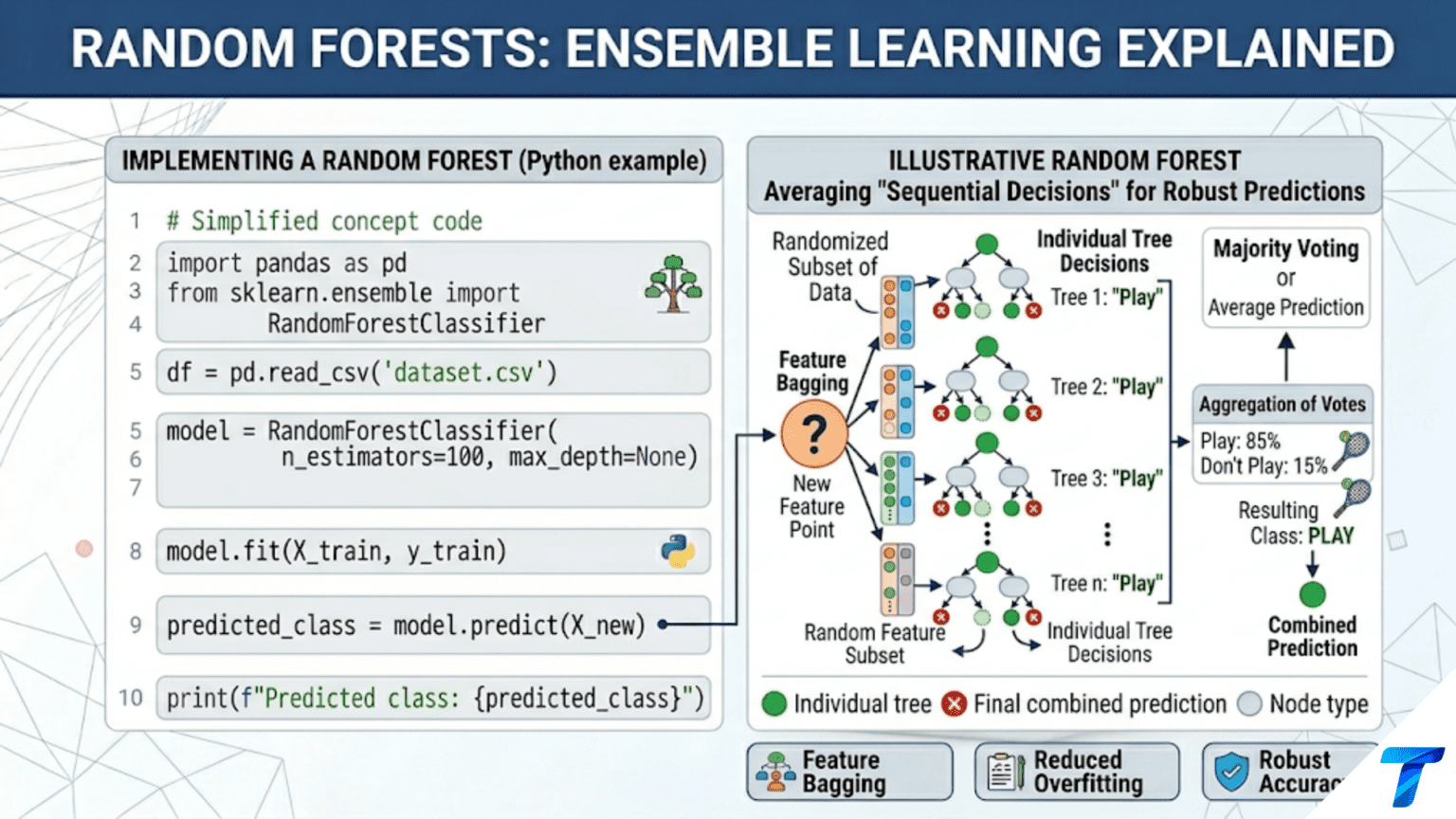
A Random Forest builds many decision trees, each trained on a random bootstrap sample of the data and considering only a random subset of features at each split. Predictions are made by majority vote (classification) or average (regression) across all trees. This combination of bagging and feature randomness reduces the high variance of individual decision trees while preserving their low bias, producing a more accurate and robust model than any single tree.
Introduction
Article 74 established the fundamental problem with single decision trees: they are highly sensitive to the specific training data they see. A small perturbation — swap out a few training examples, change a few labels — and the resulting tree can look completely different. This instability is the defining weakness of decision trees and is measured by their high variance.
The insight behind Random Forests is elegant and powerful: if individual trees are unstable, build many of them and average their predictions. The errors individual trees make tend to be uncorrelated (because each tree is trained on different data and uses different features), so their average is much more reliable than any single tree. This is the essence of ensemble learning — combining multiple weak or moderate learners into a single strong learner.
Random Forests, introduced by Leo Breiman in 2001, are the canonical example of this principle. They take an already-good algorithm (decision trees) and make it dramatically better by combining randomization with aggregation. The result is one of the most consistently strong algorithms in machine learning: robust to outliers, effective with mixed feature types, resistant to overfitting, and capable of providing reliable feature importance estimates — all without requiring feature scaling.
This article builds a complete understanding of Random Forests: the bagging technique that generates diversity, the feature randomness that ensures trees are decorrelated, the out-of-bag error estimate that provides free validation, feature importance aggregated across the ensemble, and a comprehensive comparison against single decision trees.
The Core Problem: Why Single Trees Fail
Before understanding the solution, it helps to precisely characterize the problem being solved.
Decision Tree Instability Demonstrated
import numpy as np
import matplotlib.pyplot as plt
from sklearn.datasets import make_classification, load_wine
from sklearn.tree import DecisionTreeClassifier
from sklearn.ensemble import RandomForestClassifier
from sklearn.model_selection import train_test_split, cross_val_score
from sklearn.preprocessing import StandardScaler
import warnings
warnings.filterwarnings('ignore')

np.random.seed(42)

# Generate dataset
X_base, y_base = make_classification(
    n_samples=500, n_features=20, n_informative=10,
    n_redundant=5, random_state=42
)

print("=== Decision Tree Variance: The Core Problem ===\n")
print("  Same hyperparameters, different random train-test splits:\n")
print(f"  {'Seed':>6} | {'DT Test Acc':>12} | {'RF Test Acc':>12} | "
      f"{'DT n_leaves':>12}")
print("  " + "-" * 52)

dt_accs = []
rf_accs = []

for seed in range(20):
    X_tr, X_te, y_tr, y_te = train_test_split(
        X_base, y_base, test_size=0.3, random_state=seed
    )

    dt = DecisionTreeClassifier(max_depth=5, random_state=42)
    rf = RandomForestClassifier(n_estimators=100, max_depth=5, random_state=42, n_jobs=-1)

    dt.fit(X_tr, y_tr)
    rf.fit(X_tr, y_tr)

    dt_acc = dt.score(X_te, y_te)
    rf_acc = rf.score(X_te, y_te)
    dt_accs.append(dt_acc)
    rf_accs.append(rf_acc)

    if seed < 10:
        print(f"  {seed:>6} | {dt_acc:>12.4f} | {rf_acc:>12.4f} | "
              f"{dt.get_n_leaves():>12}")

print(f"\n  Summary over 20 seeds:")
print(f"  {'Metric':<22} | {'Decision Tree':>14} | {'Random Forest':>14}")
print("  " + "-" * 54)
for label, vals in [("Mean accuracy", [np.mean(dt_accs), np.mean(rf_accs)]),
                     ("Std accuracy",  [np.std(dt_accs),  np.std(rf_accs)]),
                     ("Min accuracy",  [np.min(dt_accs),  np.min(rf_accs)]),
                     ("Max accuracy",  [np.max(dt_accs),  np.max(rf_accs)]),
                     ("Range",         [np.ptp(dt_accs),  np.ptp(rf_accs)])]:
    print(f"  {label:<22} | {vals[0]:>14.4f} | {vals[1]:>14.4f}")

print(f"\n  The Random Forest's std is {np.std(dt_accs)/np.std(rf_accs):.1f}× "
f"lower — far more stable predictions.")This demonstration isolates the variance contribution precisely. The DT and RF use the same max_depth, so their bias is similar. The dramatic reduction in standard deviation shows variance reduction at work — the core mechanism of ensemble learning.
Bootstrap Aggregation (Bagging)
The first randomization mechanism in Random Forests is bagging (Bootstrap AGGregatING), introduced by Breiman in 1994.
How Bootstrapping Works
Given a training set of n samples, a bootstrap sample is created by drawing n samples with replacement from the original dataset. This means:
- Each bootstrap sample has the same size as the original
- On average, a bootstrap sample contains approximately 63.2% of the unique original samples (the probability of any single sample being selected at least once is 1 − (1−1/n)^n → 1 − 1/e ≈ 0.632)
- The remaining ~36.8% of samples are never drawn — these are the out-of-bag (OOB) samples for this tree
Each tree in the forest trains on a different bootstrap sample, creating diversity. The variation in training data means different trees will make different errors, and when many such trees are averaged, the errors tend to cancel out.
import numpy as np

def demonstrate_bootstrapping(n_samples=1000, n_bootstrap=100, random_state=42):
    """
    Demonstrate bootstrap sampling properties:
    - Average fraction of unique samples per bootstrap
    - Distribution of sample inclusion frequencies
    - Convergence to 1 - 1/e ≈ 63.2%
    """
    np.random.seed(random_state)

    all_indices = np.arange(n_samples)

    unique_fractions  = []
    inclusion_counts  = np.zeros(n_samples, dtype=int)

    for _ in range(n_bootstrap):
        # Draw n samples with replacement
        bootstrap_idx   = np.random.choice(n_samples, size=n_samples, replace=True)
        unique_in_boot  = len(np.unique(bootstrap_idx))
        unique_fractions.append(unique_in_boot / n_samples)

        # Track how often each sample appears across all bootstraps
        for idx in np.unique(bootstrap_idx):
            inclusion_counts[idx] += 1

    print("=== Bootstrap Sampling Properties ===\n")
    print(f"  n = {n_samples:,} samples | {n_bootstrap} bootstrap replicates\n")
    print(f"  Theoretical fraction included: 1 - 1/e = {1 - 1/np.e:.4f}")
    print(f"  Observed mean fraction:        {np.mean(unique_fractions):.4f}")
    print(f"  Observed std:                  {np.std(unique_fractions):.4f}\n")

    oob_fraction = 1 - np.mean(unique_fractions)
    print(f"  Out-of-bag fraction:           {oob_fraction:.4f} (~{oob_fraction*100:.1f}%)")
    print(f"  → For each tree, ~36.8% of samples are held out for free!")

    # Show distribution of how many times each sample was drawn
    # across all 100 bootstrap replicates
    never_drawn = (inclusion_counts == 0).sum()
    print(f"\n  Samples never drawn in any bootstrap: {never_drawn}")
    print(f"  Samples drawn ≥90 times out of {n_bootstrap}: "
          f"{(inclusion_counts >= 90).sum()}")

demonstrate_bootstrapping()


def bagging_variance_reduction(n_trees_range, n_trials=50, random_state=42):
    """
    Demonstrate how variance decreases as more trees are added to the ensemble.

    For independent estimators with variance σ², the average has variance σ²/n.
    Real trees are positively correlated (ρ > 0), so actual reduction is:

        Var(ensemble) = ρ * σ² + (1-ρ) * σ²/n

    As n → ∞, Var → ρ * σ², not zero. Feature randomness reduces ρ.
    """
    np.random.seed(random_state)

    X_bv, y_bv = make_classification(
        n_samples=600, n_features=15, n_informative=8, random_state=42
    )

    mean_accs = []
    std_accs  = []

    for n_trees in n_trees_range:
        trial_accs = []
        for trial in range(n_trials):
            X_tr, X_te, y_tr, y_te = train_test_split(
                X_bv, y_bv, test_size=0.3, random_state=trial
            )
            rf = RandomForestClassifier(
                n_estimators=n_trees, random_state=42, n_jobs=-1
            )
            rf.fit(X_tr, y_tr)
            trial_accs.append(rf.score(X_te, y_te))

        mean_accs.append(np.mean(trial_accs))
        std_accs.append(np.std(trial_accs))

    fig, (ax1, ax2) = plt.subplots(1, 2, figsize=(14, 5))

    ax1.plot(n_trees_range, mean_accs, 'o-', color='steelblue', lw=2.5,
             markersize=7, label='Mean accuracy')
    ax1.fill_between(n_trees_range,
                     [m - s for m, s in zip(mean_accs, std_accs)],
                     [m + s for m, s in zip(mean_accs, std_accs)],
                     alpha=0.2, color='steelblue')
    ax1.set_xlabel('Number of Trees', fontsize=12)
    ax1.set_ylabel('Test Accuracy', fontsize=12)
    ax1.set_title('Accuracy vs Number of Trees\n(Diminishing returns after ~50-100)',
                  fontsize=11, fontweight='bold')
    ax1.legend(fontsize=10); ax1.grid(True, alpha=0.3)

    ax2.plot(n_trees_range, std_accs, 's-', color='coral', lw=2.5,
             markersize=7)
    ax2.set_xlabel('Number of Trees', fontsize=12)
    ax2.set_ylabel('Std of Test Accuracy (variance proxy)', fontsize=12)
    ax2.set_title('Variance Reduction vs Number of Trees\n'
                  '(Variance falls then plateaus at ρ·σ²)',
                  fontsize=11, fontweight='bold')
    ax2.grid(True, alpha=0.3)

    plt.suptitle('Bagging: Adding More Trees Reduces Variance',
                 fontsize=13, fontweight='bold')
    plt.tight_layout()
    plt.savefig('rf_bagging_variance.png', dpi=150)
    plt.show()
    print("Saved: rf_bagging_variance.png")


bagging_variance_reduction(
    n_trees_range=[1, 2, 3, 5, 10, 20, 50, 100, 200, 500]
)Why Averaging Reduces Variance
Suppose you have n independent classifiers, each with variance σ² and zero covariance. The variance of their average is σ²/n — averaging n independent classifiers reduces variance by a factor of n.
Real trees in a Random Forest are not independent — they are positively correlated because they all train on the same underlying distribution. For n trees with pairwise correlation ρ:
As n → ∞, this converges to ρσ² — not zero. The residual variance is controlled entirely by the tree correlation ρ. This is the fundamental insight behind the second randomization mechanism: reducing ρ through feature subsampling.
Feature Randomness: Decorrelating the Trees
If all trees were trained on the same features at each split, they would tend to select the same dominant features repeatedly. Trees grown on different bootstrap samples but always splitting on the same dominant features will still be highly correlated — limiting the variance reduction achievable by averaging.
Random Forests add a second layer of randomness: at each split, only a random subset of max_features features is considered. This forces trees to use different features even when they have bootstrap samples that overlap heavily, producing more diverse (less correlated) trees.
The default for max_features:
- Classification:
sqrt(n_features)— the square root of total feature count - Regression:
n_features / 3— one third of total features
import numpy as np
import matplotlib.pyplot as plt
from sklearn.ensemble import RandomForestClassifier
from sklearn.datasets import make_classification
from sklearn.model_selection import cross_val_score

np.random.seed(42)
X_feat, y_feat = make_classification(
    n_samples=500, n_features=20, n_informative=10, random_state=42
)

print("=== Effect of max_features on RF Performance ===\n")
print(f"  n_features = {X_feat.shape[1]}\n")
print(f"  {'max_features':>14} | {'n_features used':>16} | "
      f"{'CV Acc (mean)':>14} | {'CV Acc (std)':>13}")
print("  " + "-" * 64)

max_features_opts = [1, 2, 3, 4, 5, 7, 10, 15, 20, 'sqrt', 'log2', None]

for mf in max_features_opts:
    rf_mf = RandomForestClassifier(
        n_estimators=200, max_features=mf, random_state=42, n_jobs=-1
    )
    scores = cross_val_score(rf_mf, X_feat, y_feat, cv=5, scoring='accuracy')

    # Compute actual number of features used
    if mf == 'sqrt':
        n_used = int(np.sqrt(X_feat.shape[1]))
    elif mf == 'log2':
        n_used = int(np.log2(X_feat.shape[1]))
    elif mf is None:
        n_used = X_feat.shape[1]
    else:
        n_used = min(int(mf), X_feat.shape[1])

    best = " ← best" if mf == 'sqrt' else ""
    print(f"  {str(mf):>14} | {n_used:>16} | "
          f"{scores.mean():>14.4f} | {scores.std():>13.4f}{best}")

print(f"\n  sqrt({X_feat.shape[1]}) = {int(np.sqrt(X_feat.shape[1]))}")
print("  The default sqrt is a good starting point, but tuning helps.")


def visualize_feature_correlation(X, y, max_features_list, n_trees=50):
    """
    Estimate pairwise tree correlation for different max_features settings.
    Lower correlation = more benefit from averaging (lower ensemble variance).
    """
    from sklearn.tree import DecisionTreeClassifier

    print("\n=== Tree Correlation vs max_features ===\n")
    print("  Lower correlation = trees make more independent errors")
    print("  = more variance reduction from averaging\n")
    print(f"  {'max_features':>14} | {'Mean tree corr':>16} | {'Ensemble benefit':>17}")
    print("  " + "-" * 53)

    X_tr, X_te, y_tr, y_te = train_test_split(X, y, test_size=0.3,
                                                random_state=42)

    for mf in max_features_list:
        # Train many trees and measure their prediction correlations
        tree_preds = []

        for t in range(n_trees):
            # Bootstrap sample
            boot_idx = np.random.choice(len(X_tr), len(X_tr), replace=True)
            X_boot, y_boot = X_tr[boot_idx], y_tr[boot_idx]

            # Fit single tree with max_features
            dt = DecisionTreeClassifier(max_features=mf, random_state=t)
            dt.fit(X_boot, y_boot)
            tree_preds.append(dt.predict_proba(X_te)[:, 1])

        tree_preds = np.array(tree_preds)  # (n_trees, n_test)

        # Compute mean pairwise correlation
        corr_matrix = np.corrcoef(tree_preds)
        # Upper triangle only (exclude diagonal)
        upper_corr = corr_matrix[np.triu_indices_from(corr_matrix, k=1)]
        mean_corr  = upper_corr.mean()

        benefit = 1 / (1 - (1 - 1/n_trees) * mean_corr + 1e-8)

        print(f"  {str(mf):>14} | {mean_corr:>16.4f} | {benefit:>17.2f}×")


visualize_feature_correlation(
    X_feat, y_feat,
    max_features_list=[1, 3, 5, 10, None]
)Out-of-Bag (OOB) Error Estimation
One of the most practically useful properties of Random Forests is the out-of-bag error estimate — a free cross-validation estimate that requires no separate validation set.
Recall that each tree’s bootstrap sample excludes approximately 36.8% of training samples. These OOB samples can serve as a validation set for that specific tree: each sample is predicted only by trees whose bootstrap sample did not include it. Aggregating these predictions across all trees gives an unbiased estimate of generalization error.
import numpy as np
from sklearn.ensemble import RandomForestClassifier
from sklearn.datasets import load_breast_cancer
from sklearn.model_selection import train_test_split, cross_val_score
from sklearn.metrics import accuracy_score
import matplotlib.pyplot as plt

cancer = load_breast_cancer()
X_ca, y_ca = cancer.data, cancer.target

X_tr_ca, X_te_ca, y_tr_ca, y_te_ca = train_test_split(
    X_ca, y_ca, test_size=0.20, random_state=42, stratify=y_ca
)

print("=== Out-of-Bag Error vs Cross-Validation ===\n")

# Train RF with OOB scoring enabled
rf_oob = RandomForestClassifier(
    n_estimators=200,
    oob_score=True,         # Enable OOB scoring
    random_state=42,
    n_jobs=-1
)
rf_oob.fit(X_tr_ca, y_tr_ca)

oob_acc  = rf_oob.oob_score_
test_acc = rf_oob.score(X_te_ca, y_te_ca)

# Compare against k-fold CV
cv_scores = cross_val_score(
    RandomForestClassifier(n_estimators=200, random_state=42, n_jobs=-1),
    X_tr_ca, y_tr_ca, cv=10, scoring='accuracy'
)

print(f"  {'Estimate type':<25} | {'Accuracy':>10} | Notes")
print("  " + "-" * 55)
print(f"  {'OOB estimate':<25} | {oob_acc:>10.4f} | Free, no extra data needed")
print(f"  {'10-fold CV (mean)':<25} | {cv_scores.mean():>10.4f} | Requires {10}× retraining")
print(f"  {'10-fold CV (std)':<25} | {cv_scores.std():>10.4f} |")
print(f"  {'Hold-out test set':<25} | {test_acc:>10.4f} | Requires held-out data")

print(f"\n  OOB-Test gap: {abs(oob_acc - test_acc):.4f}")
print(f"  CV-Test gap:  {abs(cv_scores.mean() - test_acc):.4f}")
print(f"\n  OOB estimate is approximately as accurate as cross-validation")
print(f"  but comes for free during training (no additional computation).")


def oob_convergence_analysis(X, y, n_trees_range, random_state=42):
    """
    Track OOB error as trees are added to the forest.
    Shows how many trees are needed for a stable OOB estimate.
    """
    np.random.seed(random_state)
    oob_scores = []

    for n_trees in n_trees_range:
        rf = RandomForestClassifier(
            n_estimators=n_trees, oob_score=True,
            random_state=random_state, n_jobs=-1
        )
        rf.fit(X, y)
        oob_scores.append(rf.oob_score_)

    fig, ax = plt.subplots(figsize=(10, 5))
    ax.plot(n_trees_range, oob_scores, 'o-', color='steelblue',
            lw=2.5, markersize=7)
    ax.axhline(y=oob_scores[-1], color='coral', linestyle='--', lw=2,
               label=f'Converged value ≈ {oob_scores[-1]:.4f}')
    ax.set_xlabel('Number of Trees', fontsize=12)
    ax.set_ylabel('OOB Accuracy', fontsize=12)
    ax.set_title('OOB Error Convergence vs Number of Trees\n'
                 '(Stabilizes when each sample has been OOB in enough trees)',
                 fontsize=12, fontweight='bold')
    ax.legend(fontsize=10); ax.grid(True, alpha=0.3)
    plt.tight_layout()
    plt.savefig('rf_oob_convergence.png', dpi=150)
    plt.show()
    print("Saved: rf_oob_convergence.png")

    # Print convergence table
    print(f"\n  {'n_trees':>8} | {'OOB Acc':>9} | {'Change':>8}")
    print("  " + "-" * 30)
    for i, (n, acc) in enumerate(zip(n_trees_range, oob_scores)):
        change = f"{acc - oob_scores[i-1]:+.4f}" if i > 0 else "     —"
        print(f"  {n:>8} | {acc:>9.4f} | {change:>8}")


oob_convergence_analysis(
    X_tr_ca, y_tr_ca,
    n_trees_range=[5, 10, 20, 30, 50, 75, 100, 150, 200, 300, 500]
)Feature Importance in Random Forests
One of the most valuable outputs of a Random Forest is its feature importance ranking. Unlike a single decision tree where importance can be dominated by one lucky feature, the RF averages importance across hundreds of trees, producing a much more stable and reliable ranking.
Mean Decrease in Impurity (MDI)
The built-in feature importance in scikit-learn’s RandomForestClassifier is the mean decrease in impurity — averaged across all trees in the forest and all splits using each feature:
This is the same calculation as single-tree importance, but averaged across T trees. The averaging dramatically stabilizes the estimates — features that happen to get a good split by chance in one tree will not systematically win across 100 trees.
import numpy as np
import matplotlib.pyplot as plt
from sklearn.ensemble import RandomForestClassifier
from sklearn.tree import DecisionTreeClassifier
from sklearn.inspection import permutation_importance
from sklearn.datasets import load_breast_cancer
from sklearn.model_selection import train_test_split

cancer = load_breast_cancer()
X_ca, y_ca = cancer.data, cancer.target
X_tr_ca, X_te_ca, y_tr_ca, y_te_ca = train_test_split(
    X_ca, y_ca, test_size=0.25, random_state=42
)

# Compare single tree vs RF importance stability
dt_single = DecisionTreeClassifier(max_depth=5, random_state=42)
rf_model  = RandomForestClassifier(n_estimators=200, random_state=42, n_jobs=-1)

dt_single.fit(X_tr_ca, y_tr_ca)
rf_model.fit(X_tr_ca, y_tr_ca)

dt_imp = dt_single.feature_importances_
rf_imp = rf_model.feature_importances_

# Run DT 20 times with different seeds to show variance
dt_importances_all = []
for seed in range(20):
    dt_seed = DecisionTreeClassifier(max_depth=5, random_state=seed)
    dt_seed.fit(X_tr_ca, y_tr_ca)
    dt_importances_all.append(dt_seed.feature_importances_)
dt_importances_all = np.array(dt_importances_all)

fig, axes = plt.subplots(1, 3, figsize=(18, 7))

# Panel 1: Single DT importance (unstable)
sorted_idx_dt = np.argsort(dt_imp)[::-1][:15]
ax = axes[0]
ax.barh(range(15), dt_importances_all.mean(axis=0)[sorted_idx_dt],
        xerr=dt_importances_all.std(axis=0)[sorted_idx_dt],
        color='coral', edgecolor='white', error_kw={'lw': 1.5, 'ecolor': 'gray'})
ax.set_yticks(range(15))
ax.set_yticklabels([cancer.feature_names[i] for i in sorted_idx_dt], fontsize=8)
ax.set_title('Single Tree Importance\n(Mean ± std over 20 seeds — HIGH variance)',
             fontsize=10, fontweight='bold')
ax.set_xlabel('Importance', fontsize=10); ax.grid(True, alpha=0.3, axis='x')
ax.invert_yaxis()

# Panel 2: RF MDI importance (stable)
sorted_idx_rf = np.argsort(rf_imp)[::-1][:15]
ax = axes[1]

# Run RF 5 times to show its stability
rf_importances_all = []
for seed in range(5):
    rf_seed = RandomForestClassifier(n_estimators=200, random_state=seed, n_jobs=-1)
    rf_seed.fit(X_tr_ca, y_tr_ca)
    rf_importances_all.append(rf_seed.feature_importances_)
rf_importances_all = np.array(rf_importances_all)

ax.barh(range(15), rf_importances_all.mean(axis=0)[sorted_idx_rf],
        xerr=rf_importances_all.std(axis=0)[sorted_idx_rf],
        color='steelblue', edgecolor='white', error_kw={'lw': 1.5, 'ecolor': 'gray'})
ax.set_yticks(range(15))
ax.set_yticklabels([cancer.feature_names[i] for i in sorted_idx_rf], fontsize=8)
ax.set_title('Random Forest MDI Importance\n(Mean ± std over 5 RF runs — LOW variance)',
             fontsize=10, fontweight='bold')
ax.set_xlabel('Importance', fontsize=10); ax.grid(True, alpha=0.3, axis='x')
ax.invert_yaxis()

# Panel 3: RF Permutation importance
perm_imp = permutation_importance(
    rf_model, X_te_ca, y_te_ca, n_repeats=30, random_state=42, n_jobs=-1
)
sorted_idx_perm = np.argsort(perm_imp.importances_mean)[::-1][:15]
ax = axes[2]
ax.barh(range(15), perm_imp.importances_mean[sorted_idx_perm],
        xerr=perm_imp.importances_std[sorted_idx_perm],
        color='mediumseagreen', edgecolor='white',
        error_kw={'lw': 1.5, 'ecolor': 'gray'})
ax.set_yticks(range(15))
ax.set_yticklabels([cancer.feature_names[i] for i in sorted_idx_perm], fontsize=8)
ax.set_title('RF Permutation Importance\n(Unbiased, uses test data)',
             fontsize=10, fontweight='bold')
ax.set_xlabel('Accuracy drop when feature shuffled', fontsize=10)
ax.grid(True, alpha=0.3, axis='x')
ax.invert_yaxis()

plt.suptitle('Feature Importance: Single Tree vs Random Forest\n'
             'RF dramatically stabilizes importance estimates by averaging across trees',
             fontsize=13, fontweight='bold', y=1.01)
plt.tight_layout()
plt.savefig('rf_feature_importance_comparison.png', dpi=150, bbox_inches='tight')
plt.show()
print("Saved: rf_feature_importance_comparison.png")Comprehensive Random Forest vs Decision Tree Comparison
import numpy as np
import matplotlib.pyplot as plt
from sklearn.datasets import (load_iris, load_wine, load_breast_cancer,
                               make_classification, make_moons)
from sklearn.ensemble import RandomForestClassifier
from sklearn.tree import DecisionTreeClassifier
from sklearn.model_selection import (cross_val_score, RepeatedStratifiedKFold,
                                      train_test_split)
from sklearn.preprocessing import StandardScaler


def comprehensive_dt_vs_rf(datasets, n_trees=200, cv_folds=10, cv_repeats=5):
    """
    Comprehensive comparison of Decision Tree vs Random Forest
    across multiple datasets and multiple evaluation aspects.
    """
    print("=== Decision Tree vs Random Forest: Comprehensive Comparison ===\n")
    print(f"  RF uses {n_trees} trees | CV: {cv_folds}-fold × {cv_repeats} repeats\n")
    print(f"  {'Dataset':<20} | {'n':>5} | {'d':>3} | "
          f"{'DT Acc':>8} | {'DT Std':>7} | "
          f"{'RF Acc':>8} | {'RF Std':>7} | "
          f"{'RF vs DT':>9}")
    print("  " + "-" * 80)

    cv = RepeatedStratifiedKFold(n_splits=cv_folds, n_repeats=cv_repeats,
                                  random_state=42)

    results = []
    for name, (X, y) in datasets.items():
        dt = DecisionTreeClassifier(random_state=42)
        rf = RandomForestClassifier(n_estimators=n_trees, random_state=42, n_jobs=-1)

        dt_scores = cross_val_score(dt, X, y, cv=cv, scoring='accuracy', n_jobs=-1)
        rf_scores = cross_val_score(rf, X, y, cv=cv, scoring='accuracy', n_jobs=-1)

        dt_mean, dt_std = dt_scores.mean(), dt_scores.std()
        rf_mean, rf_std = rf_scores.mean(), rf_scores.std()
        improvement = rf_mean - dt_mean

        flag = (f"+{improvement*100:.1f}%" if improvement > 0.001
                else (f"{improvement*100:.1f}%" if improvement < -0.001
                      else "~equal"))

        print(f"  {name:<20} | {len(y):>5} | {X.shape[1]:>3} | "
              f"{dt_mean:>8.4f} | {dt_std:>7.4f} | "
              f"{rf_mean:>8.4f} | {rf_std:>7.4f} | "
              f"{flag:>9}")

        results.append({
            'name': name, 'n': len(y), 'd': X.shape[1],
            'dt_mean': dt_mean, 'dt_std': dt_std,
            'rf_mean': rf_mean, 'rf_std': rf_std
        })

    return results


# Prepare datasets
np.random.seed(42)
datasets_compare = {
    'Iris':          (load_iris().data,          load_iris().target),
    'Wine':          (load_wine().data,           load_wine().target),
    'Breast Cancer': (load_breast_cancer().data, load_breast_cancer().target),
    'Synthetic 20D': make_classification(500, 20, n_informative=10, random_state=42),
    'Two Moons':     make_moons(300, noise=0.25, random_state=42),
    'High-Dim 50D':  make_classification(500, 50, n_informative=15, random_state=42),
}

results = comprehensive_dt_vs_rf(datasets_compare)


def variance_vs_n_trees_visualization(X, y, n_trees_list, n_trials=50):
    """
    Show both accuracy and variance as functions of n_estimators.
    Key visualization for understanding why more trees stabilize the forest.
    """
    np.random.seed(42)

    dt_trial_accs = []
    for trial in range(n_trials):
        X_tr, X_te, y_tr, y_te = train_test_split(
            X, y, test_size=0.3, random_state=trial
        )
        dt = DecisionTreeClassifier(random_state=42)
        dt.fit(X_tr, y_tr)
        dt_trial_accs.append(dt.score(X_te, y_te))

    rf_means, rf_stds = [], []
    for n in n_trees_list:
        trial_accs = []
        for trial in range(n_trials):
            X_tr, X_te, y_tr, y_te = train_test_split(
                X, y, test_size=0.3, random_state=trial
            )
            rf = RandomForestClassifier(n_estimators=n, random_state=42, n_jobs=-1)
            rf.fit(X_tr, y_tr)
            trial_accs.append(rf.score(X_te, y_te))
        rf_means.append(np.mean(trial_accs))
        rf_stds.append(np.std(trial_accs))

    fig, (ax1, ax2) = plt.subplots(1, 2, figsize=(14, 5))

    ax1.axhline(y=np.mean(dt_trial_accs), color='coral', linestyle='--', lw=2,
                label=f'Single DT mean ({np.mean(dt_trial_accs):.3f})')
    ax1.fill_between([-0.5, len(n_trees_list) - 0.5],
                     [np.mean(dt_trial_accs) - np.std(dt_trial_accs)] * 2,
                     [np.mean(dt_trial_accs) + np.std(dt_trial_accs)] * 2,
                     alpha=0.12, color='coral')
    ax1.plot(range(len(n_trees_list)), rf_means, 'o-', color='steelblue',
             lw=2.5, markersize=8, label='RF mean accuracy')
    ax1.fill_between(range(len(n_trees_list)),
                     [m - s for m, s in zip(rf_means, rf_stds)],
                     [m + s for m, s in zip(rf_means, rf_stds)],
                     alpha=0.15, color='steelblue')
    ax1.set_xticks(range(len(n_trees_list)))
    ax1.set_xticklabels(n_trees_list, rotation=45)
    ax1.set_xlabel('Number of Trees', fontsize=12)
    ax1.set_ylabel('Test Accuracy', fontsize=12)
    ax1.set_title('RF Accuracy vs Number of Trees\n'
                  '(RF mean quickly surpasses single DT)', fontsize=11, fontweight='bold')
    ax1.legend(fontsize=10); ax1.grid(True, alpha=0.3)

    ax2.axhline(y=np.std(dt_trial_accs), color='coral', linestyle='--', lw=2,
                label=f'Single DT variance ({np.std(dt_trial_accs):.4f})')
    ax2.plot(range(len(n_trees_list)), rf_stds, 's-', color='steelblue',
             lw=2.5, markersize=8, label='RF variance')
    ax2.set_xticks(range(len(n_trees_list)))
    ax2.set_xticklabels(n_trees_list, rotation=45)
    ax2.set_xlabel('Number of Trees', fontsize=12)
    ax2.set_ylabel('Std of Test Accuracy (variance)', fontsize=12)
    ax2.set_title('RF Variance Reduction vs Number of Trees\n'
                  '(Rapid drop then plateau — diminishing returns)', fontsize=11, fontweight='bold')
    ax2.legend(fontsize=10); ax2.grid(True, alpha=0.3)

    plt.suptitle('Random Forest: Accuracy and Variance vs Number of Trees',
                 fontsize=13, fontweight='bold')
    plt.tight_layout()
    plt.savefig('rf_accuracy_variance_n_trees.png', dpi=150)
    plt.show()
    print("Saved: rf_accuracy_variance_n_trees.png")


wine = load_wine()
variance_vs_n_trees_visualization(
    wine.data, wine.target,
    n_trees_list=[1, 2, 5, 10, 25, 50, 100, 200, 500]
)Hyperparameters and Tuning Guide
Random Forests have several hyperparameters, but most problems are solved well with defaults or a small search over the two most impactful parameters.
The Most Important Parameters
import numpy as np
from sklearn.ensemble import RandomForestClassifier
from sklearn.datasets import load_breast_cancer
from sklearn.model_selection import GridSearchCV, StratifiedKFold

cancer = load_breast_cancer()
X_ca, y_ca = cancer.data, cancer.target

print("=== Random Forest Hyperparameter Guide ===\n")
print("  Key parameters (roughly in order of impact):\n")

param_table = [
    ("n_estimators",    "100–500",   "More = lower variance, diminishing returns after ~200"),
    ("max_features",    "sqrt/log2", "Controls tree correlation; tune first for RF"),
    ("max_depth",       "None/10-30","None (no limit) usually best; limit to reduce overfit"),
    ("min_samples_leaf","1–10",      "Higher = more regularization, less overfit on small data"),
    ("min_samples_split","2–20",     "Higher = more regularization"),
    ("max_samples",     "0.5–1.0",   "Bootstrap sample size fraction (usually leave at 1.0)"),
    ("class_weight",    "balanced",  "For imbalanced data; adjusts class penalties"),
]

print(f"  {'Parameter':<22} | {'Typical range':>15} | Notes")
print("  " + "-" * 75)
for param, rng, note in param_table:
    print(f"  {param:<22} | {rng:>15} | {note}")


# Targeted hyperparameter search on the two most impactful parameters
cv_tune = StratifiedKFold(n_splits=5, shuffle=True, random_state=42)

param_grid = {
    'n_estimators':     [100, 200, 300],
    'max_features':     ['sqrt', 'log2', 0.3, 0.5],
    'max_depth':        [None, 10, 20],
    'min_samples_leaf': [1, 2, 5],
}

rf_tune = RandomForestClassifier(random_state=42, n_jobs=-1)
grid_search = GridSearchCV(
    rf_tune, param_grid, cv=cv_tune,
    scoring='roc_auc', n_jobs=-1, verbose=0,
    return_train_score=False
)

grid_search.fit(X_ca, y_ca)

print(f"\n  Best parameters found:")
for param, val in grid_search.best_params_.items():
    print(f"    {param}: {val}")
print(f"\n  Best CV AUC: {grid_search.best_score_:.4f}")

# Show top 10 configurations
import pandas as pd
cv_results = pd.DataFrame(grid_search.cv_results_)
top_10 = (cv_results[['param_n_estimators', 'param_max_features',
                        'param_max_depth', 'param_min_samples_leaf',
                        'mean_test_score', 'std_test_score']]
           .sort_values('mean_test_score', ascending=False)
           .head(10))

print(f"\n  Top 10 configurations:\n")
print(f"  {'n_est':>6} | {'max_feat':>10} | {'max_d':>7} | "
      f"{'min_leaf':>9} | {'AUC':>8} | {'±':>7}")
print("  " + "-" * 58)
for _, row in top_10.iterrows():
    print(f"  {int(row['param_n_estimators']):>6} | "
          f"{str(row['param_max_features']):>10} | "
          f"{str(row['param_max_depth']):>7} | "
          f"{int(row['param_min_samples_leaf']):>9} | "
          f"{row['mean_test_score']:>8.4f} | "
f"{row['std_test_score']:>7.4f}")Decision Boundary Comparison: Tree vs Forest
A direct visual comparison of single-tree and Random Forest decision boundaries reveals the mechanism of variance reduction in a way that numbers alone cannot.
import numpy as np
import matplotlib.pyplot as plt
from sklearn.tree import DecisionTreeClassifier
from sklearn.ensemble import RandomForestClassifier
from sklearn.datasets import make_moons, make_classification
from sklearn.model_selection import train_test_split
from matplotlib.colors import ListedColormap


def compare_boundaries(X_train, y_train, X_test, y_test,
                         title="Decision Tree vs Random Forest",
                         figsize=(18, 5)):
    """
    Side-by-side boundary comparison:
    1. Single deep DT (high variance, complex boundary)
    2. Single shallow DT (high bias, simple boundary)
    3. Random Forest (smooth, stable boundary)
    4. Uncertainty map — where does RF confidence drop below 70%?
    """
    x_min, x_max = X_train[:, 0].min() - 0.5, X_train[:, 0].max() + 0.5
    y_min, y_max = X_train[:, 1].min() - 0.5, X_train[:, 1].max() + 0.5
    xx, yy = np.meshgrid(np.linspace(x_min, x_max, 250),
                          np.linspace(y_min, y_max, 250))
    grid = np.c_[xx.ravel(), yy.ravel()]

    # Fit models
    dt_deep   = DecisionTreeClassifier(max_depth=None, random_state=42)
    dt_shallow = DecisionTreeClassifier(max_depth=3, random_state=42)
    rf         = RandomForestClassifier(n_estimators=200, random_state=42, n_jobs=-1)

    dt_deep.fit(X_train, y_train)
    dt_shallow.fit(X_train, y_train)
    rf.fit(X_train, y_train)

    Z_deep    = dt_deep.predict(grid).reshape(xx.shape)
    Z_shallow = dt_shallow.predict(grid).reshape(xx.shape)
    Z_rf      = rf.predict(grid).reshape(xx.shape)
    P_rf      = rf.predict_proba(grid)[:, 1].reshape(xx.shape)

    palette_bg  = ['#d0e8f8', '#f8d0d0']
    palette_pts = ['steelblue', 'coral']
    cmap_bg     = ListedColormap(palette_bg)

    fig, axes = plt.subplots(1, 4, figsize=figsize)

    configs = [
        (Z_deep,    dt_deep,    "Single DT (no depth limit)\n"
                                 f"Leaves={dt_deep.get_n_leaves()} | "
                                 f"Test={dt_deep.score(X_test, y_test):.3f}"),
        (Z_shallow, dt_shallow, "Single DT (depth=3)\n"
                                 f"Leaves={dt_shallow.get_n_leaves()} | "
                                 f"Test={dt_shallow.score(X_test, y_test):.3f}"),
        (Z_rf,      rf,         "Random Forest (200 trees)\n"
                                 f"Test={rf.score(X_test, y_test):.3f}"),
    ]

    for ax, (Z, model, label) in zip(axes[:3], configs):
        ax.contourf(xx, yy, Z, alpha=0.35, cmap=cmap_bg)
        ax.contour(xx, yy, Z, colors='black', linewidths=0.8, alpha=0.4)
        for cls, color in zip([0, 1], palette_pts):
            mask = y_train == cls
            ax.scatter(X_train[mask, 0], X_train[mask, 1], c=color,
                       edgecolors='white', s=35, linewidth=0.4, alpha=0.85)
        ax.set_title(label, fontsize=9, fontweight='bold')
        ax.set_xlabel('Feature 1', fontsize=9)
        ax.grid(True, alpha=0.2)

    # Panel 4: RF uncertainty map
    ax = axes[3]
    uncertainty = 1 - np.abs(P_rf - 0.5) * 2  # 0=certain, 1=uncertain
    im = ax.contourf(xx, yy, uncertainty, levels=20, cmap='RdYlGn_r', alpha=0.8)
    plt.colorbar(im, ax=ax, label='Uncertainty')
    ax.contour(xx, yy, Z_rf, colors='black', linewidths=0.8, alpha=0.3)
    for cls, color in zip([0, 1], palette_pts):
        mask = y_test == cls
        ax.scatter(X_test[mask, 0], X_test[mask, 1], c=color,
                   edgecolors='white', s=35, linewidth=0.4, alpha=0.85)
    ax.set_title("RF Uncertainty Map\n(Red=uncertain, Green=confident)",
                 fontsize=9, fontweight='bold')
    ax.set_xlabel('Feature 1', fontsize=9)
    ax.grid(True, alpha=0.2)

    plt.suptitle(title, fontsize=12, fontweight='bold', y=1.02)
    plt.tight_layout()
    plt.savefig('rf_vs_dt_boundaries.png', dpi=150, bbox_inches='tight')
    plt.show()
    print("Saved: rf_vs_dt_boundaries.png")


np.random.seed(42)
X_mns, y_mns = make_moons(n_samples=400, noise=0.30, random_state=42)
X_tr_mns, X_te_mns, y_tr_mns, y_te_mns = train_test_split(
    X_mns, y_mns, test_size=0.25, random_state=42
)

compare_boundaries(
    X_tr_mns, y_tr_mns, X_te_mns, y_te_mns,
    title="Decision Boundary Comparison: Two Moons Dataset\n"
          "(Deep DT memorizes, shallow DT misses curve, RF finds the right balance)"
)The boundary comparison reveals three qualitatively different behaviors. The unconstrained single tree produces a jagged, irregular boundary that follows every quirk in the training data — perfect training accuracy, mediocre test accuracy, and a boundary that would change substantially with a different training sample. The shallow tree is stable but misses the true curved boundary. The Random Forest boundary is smooth, stable, and closely follows the true moon-shaped boundary — the averaging of many imperfect trees cancels out individual quirks and produces a boundary that generalizes well.
The uncertainty map (fourth panel) adds another dimension: the RF can quantify its own confidence. Regions near the true decision boundary show higher uncertainty (red), while regions clearly belonging to one class show high confidence (green). This uncertainty estimate is a major practical advantage — it allows the model to flag ambiguous predictions for human review.
Proximity Matrix: Understanding What RF Learns
Beyond predictions and importances, a Random Forest implicitly defines a proximity matrix between samples: two samples are “close” if they land in the same leaf in many trees. This proximity measure is learned from the data structure itself rather than from any predefined distance metric.
import numpy as np
import matplotlib.pyplot as plt
from sklearn.ensemble import RandomForestClassifier
from sklearn.datasets import load_iris

def compute_rf_proximity(rf, X):
    """
    Compute the Random Forest proximity matrix.

    Two samples i and j are proximate if they land in the same leaf
    in many trees. Proximity = (number of trees where i and j co-occur)
    divided by (total number of trees).

    Useful for:
    - Detecting mislabeled samples (proximate to other-class samples)
    - Imputing missing values (use proximate samples as donors)
    - Unsupervised learning and clustering

    Args:
        rf: Fitted RandomForestClassifier or Regressor
        X:  Feature matrix, shape (n_samples, n_features)

    Returns:
        Proximity matrix, shape (n_samples, n_samples), values in [0, 1]
    """
    n_samples = X.shape[0]
    n_trees   = len(rf.estimators_)

    # Get leaf node for each sample in each tree
    # apply() returns shape (n_samples, n_trees)
    leaf_indices = rf.apply(X)

    proximity = np.zeros((n_samples, n_samples))

    for tree_idx in range(n_trees):
        leaves = leaf_indices[:, tree_idx]
        # For each pair of samples in the same leaf, increment proximity
        for leaf_id in np.unique(leaves):
            in_leaf = np.where(leaves == leaf_id)[0]
            if len(in_leaf) > 1:
                # All pairs within this leaf get +1
                pairs = np.ix_(in_leaf, in_leaf)
                proximity[pairs] += 1

    # Normalize by number of trees
    proximity /= n_trees
    # Zero diagonal (self-proximity is trivially 1 but uninformative)
    np.fill_diagonal(proximity, 0)

    return proximity


# Compute proximity on Iris
iris = load_iris()
X_ir, y_ir = iris.data, iris.target

rf_prox = RandomForestClassifier(n_estimators=500, random_state=42, n_jobs=-1)
rf_prox.fit(X_ir, y_ir)

print("Computing RF proximity matrix...")
prox_matrix = compute_rf_proximity(rf_prox, X_ir)

# Visualize the proximity matrix sorted by class
sort_idx = np.argsort(y_ir)
prox_sorted = prox_matrix[sort_idx][:, sort_idx]
y_sorted    = y_ir[sort_idx]

fig, axes = plt.subplots(1, 2, figsize=(14, 6))

im = axes[0].imshow(prox_sorted, cmap='viridis', aspect='auto')
plt.colorbar(im, ax=axes[0], label='Proximity')

# Draw class boundaries
class_boundaries = [0]
for c in range(3):
    class_boundaries.append(class_boundaries[-1] + (y_sorted == c).sum())

for b in class_boundaries[1:-1]:
    axes[0].axhline(y=b - 0.5, color='white', lw=2)
    axes[0].axvline(x=b - 0.5, color='white', lw=2)

axes[0].set_title('RF Proximity Matrix: Iris Dataset\n'
                   '(Sorted by class — bright = proximate in the forest)',
                   fontsize=11, fontweight='bold')
axes[0].set_xlabel('Sample index (sorted by class)', fontsize=10)
axes[0].set_ylabel('Sample index (sorted by class)', fontsize=10)

# Label class regions
cumulative = 0
for c, name in enumerate(iris.target_names):
    count = (y_sorted == c).sum()
    axes[0].text(cumulative + count/2, cumulative + count/2,
                 name, ha='center', va='center',
                 fontsize=9, color='white', fontweight='bold',
                 bbox=dict(boxstyle='round', fc='black', alpha=0.4))
    cumulative += count

# Show proximity to a specific sample
sample_id = 75  # A versicolor sample near the boundary
prox_to_sample = prox_matrix[sample_id]

# Sort by proximity
sorted_prox_idx = np.argsort(prox_to_sample)[::-1][:30]

colors = ['steelblue', 'coral', 'mediumseagreen']
bar_colors = [colors[y_ir[i]] for i in sorted_prox_idx]

axes[1].bar(range(30), prox_to_sample[sorted_prox_idx],
            color=bar_colors, edgecolor='white', linewidth=0.5)
axes[1].set_xlabel('Rank of Nearest Neighbors', fontsize=11)
axes[1].set_ylabel('Proximity Score', fontsize=11)
axes[1].set_title(f'Proximity to Sample #{sample_id} '
                   f'(Class: {iris.target_names[y_ir[sample_id]]})\n'
                   f'Blue=setosa, Red=versicolor, Green=virginica',
                   fontsize=11, fontweight='bold')
axes[1].grid(True, alpha=0.3, axis='y')

plt.suptitle('Random Forest Proximity: A Learned Similarity Measure',
             fontsize=13, fontweight='bold')
plt.tight_layout()
plt.savefig('rf_proximity_matrix.png', dpi=150, bbox_inches='tight')
plt.show()
print("Saved: rf_proximity_matrix.png")

print(f"\n  Sample #{sample_id} (Class: {iris.target_names[y_ir[sample_id]]})")
print(f"  Top 5 most proximate samples:")
for rank, idx in enumerate(sorted_prox_idx[:5], 1):
    print(f"    {rank}. Sample #{idx} (Class: {iris.target_names[y_ir[idx]]}) "
          f"Proximity = {prox_to_sample[idx]:.4f}")
Random Forests for Regression
Everything above applies to classification. For regression, the Random Forest Regressor averages the predicted values across all trees (instead of majority voting) and uses variance reduction as the splitting criterion.
import numpy as np
import matplotlib.pyplot as plt
from sklearn.ensemble import RandomForestRegressor
from sklearn.tree import DecisionTreeRegressor
from sklearn.datasets import fetch_california_housing
from sklearn.model_selection import cross_val_score
from sklearn.metrics import mean_squared_error, r2_score

housing = fetch_california_housing()
X_h, y_h = housing.data, housing.target

print("=== Random Forest Regression: California Housing ===\n")
print(f"  {'Model':<30} | {'CV R²':>9} | {'CV RMSE':>9} | Notes")
print("  " + "-" * 65)

models = [
    ("Decision Tree (max_d=5)",  DecisionTreeRegressor(max_depth=5, random_state=42)),
    ("Decision Tree (max_d=10)", DecisionTreeRegressor(max_depth=10, random_state=42)),
    ("Decision Tree (no limit)", DecisionTreeRegressor(random_state=42)),
    ("RF (100 trees)",           RandomForestRegressor(n_estimators=100, random_state=42, n_jobs=-1)),
    ("RF (200 trees)",           RandomForestRegressor(n_estimators=200, random_state=42, n_jobs=-1)),
    ("RF (max_d=10)",            RandomForestRegressor(n_estimators=200, max_depth=10,
                                                         random_state=42, n_jobs=-1)),
]

for name, model in models:
    r2_scores   = cross_val_score(model, X_h, y_h, cv=5, scoring='r2', n_jobs=-1)
    rmse_scores = np.sqrt(-cross_val_score(model, X_h, y_h, cv=5,
                                            scoring='neg_mean_squared_error', n_jobs=-1))

    flag = " ← best" if "RF (200" in name else ""
print(f" {name:<30} | {r2_scores.mean():>9.4f} | {rmse_scores.mean():>9.4f} |{flag}")When to Use Random Forests (and When Not To)
Use Random Forests when:
You need a strong default. Random Forests with default hyperparameters perform well on most tabular datasets without any tuning. They are the best single algorithm to try first on a new tabular problem.
Interpretability is secondary to accuracy. A 200-tree forest cannot be explained as a sequence of rules the way a single shallow tree can. If stakeholders need to follow the model’s logic rule-by-rule, a single constrained tree or a linear model is more appropriate.
Features are mixed or messy. Random Forests handle numerical and categorical features (after encoding), missing value proxies, skewed distributions, and correlated features all without preprocessing. They do not need scaling.
You want built-in feature importance. The forest provides a stable, aggregated feature importance ranking at no extra cost.
You need calibrated OOB performance estimates. The OOB error eliminates the need for a separate validation set, useful when data is limited.
Be cautious when:
Training data is very small. With fewer than ~200 samples, bootstrap samples overlap heavily and the diversity benefit of multiple trees diminishes.
Real-time prediction latency is critical. Predicting with 500 trees takes 500× longer than predicting with one tree. For sub-millisecond serving, consider lighter alternatives.
Extrapolation is required. Like single trees, Random Forest regressors cannot extrapolate beyond the range of training target values — they plateau at the training data boundary.
High-dimensional sparse data (text, images). Random Forests struggle with sparse, very high-dimensional data (e.g., TF-IDF bag-of-words with 50,000 features). Gradient boosting or neural networks typically perform better in these settings.
Summary
Random Forests solve the fundamental problem of decision trees — high variance — by combining two orthogonal sources of randomization: bootstrap sampling (bagging) to create different training sets for each tree, and feature subsampling to ensure the trees are not all dominated by the same strong features. The predictions of many such decorrelated trees, when averaged, have dramatically lower variance while preserving similar bias to individual trees.
The mathematical principle is clean: for n trees with pairwise correlation ρ and individual variance σ², the ensemble variance is ρσ² + (1-ρ)σ²/n. As n grows, variance approaches ρσ² — the minimum achievable with n trees. Reducing ρ (the tree correlation) through feature subsampling is therefore the key lever beyond simply adding more trees.
Practical implications follow directly from this theory: the OOB error provides free reliable performance estimates; feature importances averaged across many trees are far more stable than single-tree importances; more trees always help but with diminishing returns; and the two most impactful hyperparameters to tune are max_features (controls ρ) and n_estimators (controls the 1/n term).
Random Forests remain one of the most reliable algorithms for tabular machine learning — frequently competitive with gradient boosted trees, simpler to tune, and faster to train. Understanding their mechanics deeply is prerequisite knowledge for understanding the ensemble methods that extend them: bagging, gradient boosting, and stacking all build on the same core insight that combining diverse imperfect models outperforms any single model.