Designing voltage dividers for sensor reading applications involves selecting a fixed resistor value that maximizes the output voltage range across the sensor’s resistance range, ensures the ADC input stays within safe limits, provides adequate resolution at the region of interest, minimizes power consumption, and accounts for loading effects from the measurement device. The optimal fixed resistor typically equals the geometric mean of the sensor’s minimum and maximum resistance values, creating the widest voltage swing and best sensitivity for accurate analog-to-digital conversion.
Introduction: Converting Resistance to Voltage
Resistive sensors—thermistors, photoresistors, potentiometers, strain gauges, flex sensors, and countless others—change their resistance in response to physical phenomena. But microcontrollers and data acquisition systems can’t measure resistance directly; they measure voltage through analog-to-digital converters (ADCs). This creates a fundamental challenge: how do you convert a changing resistance into a voltage that your system can read accurately?
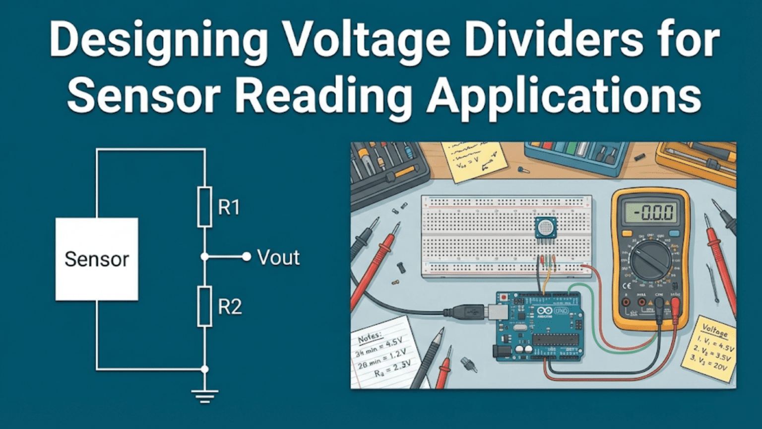
The voltage divider circuit provides the classic solution. By placing the sensor as one resistor in a divider configuration and choosing the other resistor carefully, you create a circuit where resistance changes translate to voltage changes. Yet this seemingly simple task involves numerous design considerations that separate amateur implementations from professional-quality sensor interfaces.
A poorly designed sensor divider exhibits problems: limited voltage swing that wastes ADC resolution, non-linear response that complicates calibration, excessive noise susceptibility from high impedance, power consumption that drains batteries, or inadequate sensitivity in the operating range you care about. A well-designed sensor divider maximizes useful voltage range, provides linear response where needed, minimizes power consumption, and delivers clean signals that translate to accurate measurements.
The difference between these outcomes lies in understanding the principles behind sensor divider design. You need to know how to select the optimal fixed resistor value, when to place the sensor on top versus bottom of the divider, how to maximize voltage swing across your sensor’s operating range, how to deal with nonlinear sensors, and how to optimize for different ADC characteristics and power constraints.
This comprehensive guide takes you through the entire design process for sensor voltage dividers. We’ll explore the theory behind optimal resistor selection, work through detailed design examples for different sensor types, examine techniques for maximizing sensitivity and linearity, investigate noise and power considerations, and develop practical design strategies for real-world applications.
Whether you’re interfacing a simple temperature sensor to an Arduino or designing a precision data acquisition system for industrial sensors, understanding these principles will help you create sensor interfaces that deliver accurate, reliable measurements.
Let’s begin by understanding the fundamental challenge of sensor interfacing and why voltage dividers are the standard solution.
The Sensor Interfacing Challenge
Why Resistive Sensors Need Voltage Dividers
The fundamental problem: Microcontrollers and ADCs measure voltage, not resistance.
Resistive sensors provide: A resistance that varies with the measured quantity
- Thermistors: Resistance varies with temperature
- Photoresistors (LDRs): Resistance varies with light intensity
- Potentiometers: Resistance varies with position
- Strain gauges: Resistance varies with mechanical strain
- Flex sensors: Resistance varies with bending
- Humidity sensors: Resistance varies with humidity
What we need: A voltage that varies proportionally (or at least predictably) with the measured quantity.
The voltage divider solution:
V_supply ----[R_fixed]----+---- V_out to ADC
                          |
                     [R_sensor]
                          |
GNDAs R_sensor changes, the voltage division ratio changes, producing V_out that varies with the measured quantity.
The Basic Conversion: Resistance to Voltage
Voltage divider formula: V_out = V_supply × (R_sensor / (R_fixed + R_sensor))
What this tells us:
- When R_sensor increases, V_out increases (sensor on bottom)
- When R_sensor decreases, V_out decreases (sensor on bottom)
- The relationship is nonlinear (we’ll address this)
- The rate of voltage change depends on the ratio of R_fixed to R_sensor
Alternative configuration (sensor on top):
V_supply ----[R_sensor]----+---- V_out to ADC
                           |
                        [R_fixed]
                           |
GNDV_out = V_supply × (R_fixed / (R_sensor + R_fixed))
Now when R_sensor increases, V_out decreases (inverse relationship).
Key Design Objectives
When designing a sensor voltage divider, we typically want to:
- Maximize voltage swing: Use as much of the ADC’s input range as possible
- Optimize sensitivity: Ensure adequate voltage change per unit of sensor change
- Minimize power consumption: Especially critical for battery-powered applications
- Provide adequate resolution: Voltage changes should exceed ADC resolution
- Ensure linearity (if needed): For some applications, linear response is important
- Minimize noise susceptibility: Low impedance reduces noise pickup
- Avoid loading effects: Divider impedance should be compatible with ADC input impedance
These objectives often conflict, requiring engineering trade-offs based on application requirements.
Selecting the Optimal Fixed Resistor Value
The Geometric Mean Principle
For maximum voltage swing across a sensor’s resistance range, the optimal fixed resistor value is the geometric mean of the sensor’s minimum and maximum resistance:
R_fixed_optimal = √(R_min × R_max)
Where:
- R_min is the sensor’s minimum resistance
- R_max is the sensor’s maximum resistance
Why this works: The geometric mean creates the most symmetrical voltage swing around the midpoint voltage.
Example: Thermistor ranges from 2kΩ to 50kΩ R_fixed_optimal = √(2,000 × 50,000) = √100,000,000 = 10kΩ
Verification: At R_min = 2kΩ with 5V supply: V_out = 5V × (2kΩ / 12kΩ) ≈ 0.83V
At R_max = 50kΩ: V_out = 5V × (50kΩ / 60kΩ) ≈ 4.17V
Voltage swing: 4.17V – 0.83V = 3.34V (uses 67% of 5V range)
Calculating Voltage Swing for Different R_fixed Values
Let’s see how different fixed resistor values affect voltage swing:
Sensor: 2kΩ to 50kΩ (25:1 range) Supply: 5V Configuration: Sensor on bottom
Case 1: R_fixed = 2kΩ (equals R_min) V_min = 5V × (2kΩ / 4kΩ) = 2.5V V_max = 5V × (50kΩ / 52kΩ) = 4.81V Swing = 2.31V
Case 2: R_fixed = 10kΩ (geometric mean) V_min = 5V × (2kΩ / 12kΩ) = 0.83V V_max = 5V × (50kΩ / 60kΩ) = 4.17V Swing = 3.34V ✓ (maximum!)
Case 3: R_fixed = 50kΩ (equals R_max) V_min = 5V × (2kΩ / 52kΩ) = 0.19V V_max = 5V × (50kΩ / 100kΩ) = 2.5V Swing = 2.31V
Conclusion: Geometric mean provides maximum swing (3.34V vs. 2.31V for other choices).
Practical Considerations in Resistor Selection
Standard values: The calculated geometric mean may not be a standard resistor value.
Example: √(1kΩ × 47kΩ) = √47,000,000 ≈ 6.86kΩ
Nearest standard values: 6.8kΩ or 7.5kΩ
Either works well; calculate swing for both:
With 6.8kΩ: V_swing = [5V × 47kΩ/(47kΩ+6.8kΩ)] – [5V × 1kΩ/(1kΩ+6.8kΩ)] = 4.37V – 0.64V = 3.73V
With 7.5kΩ: V_swing = [5V × 47kΩ/(47kΩ+7.5kΩ)] – [5V × 1kΩ/(1kΩ+7.5kΩ)] = 4.31V – 0.59V = 3.72V
Both nearly identical; choose based on availability.
Optimizing for Region of Interest
Important principle: You don’t always care about the entire sensor range equally.
Example: Room temperature thermistor
- Sensor range: -40°C to +125°C (1MΩ to 100Ω)
- Region of interest: 15°C to 30°C (50kΩ to 20kΩ)
Option 1: Optimize for full range R_fixed = √(100Ω × 1MΩ) = 10kΩ This gives good overall range but mediocre sensitivity in 15-30°C range.
Option 2: Optimize for 15-30°C R_fixed = √(20kΩ × 50kΩ) ≈ 31.6kΩ (use 33kΩ) This maximizes voltage swing in the temperature range you actually care about.
Trade-off: Reduced swing at extreme temperatures, but better resolution where it matters.
Power Consumption Considerations
The fixed resistor value determines current draw from the power supply:
Current through divider: I = V_supply / (R_fixed + R_sensor)
Power consumption: P = V_supply × I = V_supply² / (R_fixed + R_sensor)
Example: 5V supply, 10kΩ fixed, sensor varies 2kΩ to 50kΩ
Maximum current (sensor at minimum): I_max = 5V / (10kΩ + 2kΩ) ≈ 0.42mA P_max = 5V × 0.42mA ≈ 2.1mW
Minimum current (sensor at maximum): I_min = 5V / (10kΩ + 50kΩ) ≈ 0.083mA P_min = 5V × 0.083mA ≈ 0.42mW
For battery-powered applications: Higher resistance values (100kΩ, 1MΩ) reduce power consumption but increase susceptibility to noise and loading effects.
Trade-off strategy:
- Low power critical: Use highest practical R_fixed (100kΩ-1MΩ)
- Noise immunity critical: Use lowest practical R_fixed (1kΩ-10kΩ)
- Balanced design: 10kΩ-100kΩ range
Design Process: Step-by-Step
Step 1: Characterize the Sensor
Gather key specifications:
- Resistance range: R_min to R_max
- Operating conditions: Temperature, humidity, etc.
- Tolerance: ±% variation between units
- Response time: How quickly resistance changes
- Power rating: Maximum safe power dissipation
Example: NTC Thermistor
- Part number: 103AT-2 (hypothetical)
- Nominal: 10kΩ at 25°C
- Range of interest: 0°C to 50°C
- R at 0°C: ≈27.3kΩ
- R at 50°C: ≈3.9kΩ
- Tolerance: ±5%
Step 2: Define Requirements
Specify design requirements:
- Measurement range: What physical quantity range?
- Resolution needed: Smallest measurable change
- ADC characteristics: Voltage range, bit depth, impedance
- Power budget: Maximum acceptable current draw
- Environmental conditions: Temperature range, noise environment
- Response time: How fast must system respond?
Example Requirements:
- Measure temperature: 0°C to 50°C
- Resolution: ±0.5°C
- ADC: 10-bit (1024 steps), 0-5V, 100kΩ input impedance
- Power: <1mA average
- Environment: Indoor, moderate electrical noise
- Response: <10 seconds acceptable
Step 3: Calculate Optimal Fixed Resistor
Using geometric mean: R_fixed = √(R_min × R_max) R_fixed = √(3,900Ω × 27,300Ω) R_fixed = √106,470,000 ≈ 10,318Ω
Select nearest standard value: 10kΩ
Step 4: Verify Voltage Range
Calculate voltage at extremes:
At 0°C (R = 27.3kΩ): V_out = 5V × (27.3kΩ / 37.3kΩ) ≈ 3.66V
At 50°C (R = 3.9kΩ): V_out = 5V × (3.9kΩ / 13.9kΩ) ≈ 1.40V
Voltage swing: 3.66V – 1.40V = 2.26V
Check ADC utilization: 2.26V / 5V = 45.2% of ADC range (acceptable, not great)
Could we improve? Try larger R_fixed to shift range:
With R_fixed = 15kΩ: At 0°C: V_out = 5V × (27.3kΩ / 42.3kΩ) ≈ 3.23V At 50°C: V_out = 5V × (3.9kΩ / 18.9kΩ) ≈ 1.03V Swing = 2.20V (slightly worse)
Stick with 10kΩ.
Step 5: Calculate Resolution
ADC resolution: 5V / 1024 steps = 4.88mV per step
Temperature per ADC step: Need to account for nonlinear thermistor response. At midpoint (25°C, ~10kΩ):
Thermistor sensitivity: Approximately -4% per °C (NTC) ΔR ≈ 10kΩ × 0.04 = 400Ω per °C
Voltage change per °C at 25°C: At 25°C: V_out = 5V × (10kΩ / 20kΩ) = 2.5V
At 26°C (R ≈ 9.6kΩ): V_out = 5V × (9.6kΩ / 19.6kΩ) ≈ 2.45V
ΔV per °C ≈ 50mV (at 25°C)
ADC steps per °C: 50mV / 4.88mV ≈ 10 steps
Actual resolution: 0.1°C (exceeds 0.5°C requirement) ✓
Step 6: Check Power Consumption
Maximum current (at 50°C, lowest resistance): I_max = 5V / (10kΩ + 3.9kΩ) ≈ 0.36mA
Well below 1mA requirement ✓
Step 7: Verify Loading Effects
ADC input impedance: 100kΩ
Equivalent R₂ (sensor on bottom) at worst case: Sensor at maximum (27.3kΩ) in parallel with ADC (100kΩ): R_eq = (27.3kΩ × 100kΩ) / 127.3kΩ ≈ 21.4kΩ
Voltage error: Unloaded: V = 5V × (27.3kΩ / 37.3kΩ) = 3.66V Loaded: V = 5V × (21.4kΩ / 31.4kΩ) = 3.41V
Error: (3.66V – 3.41V) / 3.66V ≈ 6.8%
This is significant! Need to either:
- Account for in software calibration
- Use lower R_fixed (more power consumption)
- Add buffer amplifier
Decision: Software calibration acceptable for this application.
Sensor-Specific Design Examples
Example 1: Photoresistor (LDR) Light Sensor
Sensor characteristics:
- Bright light: 100Ω
- Dim light: 1MΩ
- Typical room light: 5kΩ-20kΩ
- Power rating: 100mW max
Requirements:
- Measure room light levels primarily
- 8-bit ADC (256 steps), 0-3.3V
- Battery powered, minimize current
- Arduino analog input (high impedance)
Design:
Step 1: Region of interest optimization Care about 5kΩ to 20kΩ (room lighting): R_fixed = √(5kΩ × 20kΩ) = √100,000,000 = 10kΩ
Step 2: Calculate voltage range Configuration: Sensor on bottom (voltage increases with more light)
3.3V ----[10kΩ]----+---- V_out
                   |
                 [LDR]
                   |
GNDAt bright (100Ω): V_out = 3.3V × (100Ω / 10.1kΩ) ≈ 0.033V
At dim (1MΩ): V_out = 3.3V × (1MΩ / 1.01MΩ) ≈ 3.27V
Full range: 0.033V to 3.27V (excellent use of ADC range!)
In region of interest: At 5kΩ: V_out = 3.3V × (5kΩ / 15kΩ) = 1.1V At 20kΩ: V_out = 3.3V × (20kΩ / 30kΩ) = 2.2V
Room light range: 1.1V to 2.2V (88 ADC steps, adequate resolution)
Step 3: Power consumption At brightest (worst case): I = 3.3V / 10.1kΩ ≈ 0.33mA P = 3.3V × 0.33mA ≈ 1.1mW (acceptable for battery)
Final design: 10kΩ fixed resistor, sensor on bottom
Example 2: Potentiometer Position Sensor
Sensor characteristics:
- 10kΩ linear potentiometer
- Rotation: 0° to 300° (270° usable)
- Used for user input (volume control, brightness, etc.)
Requirements:
- Full 0-5V output range across rotation
- 10-bit ADC (Arduino)
- Smooth, linear response
- No power consumption concern (USB powered)
Design:
This is unique because a potentiometer is already a voltage divider!
Configuration:
5V ---- [POT] ---- 0V
          |
Wiper (to ADC)The potentiometer itself creates perfect voltage division:
- At 0°: V_out = 0V
- At 150° (mid-rotation): V_out = 2.5V
- At 300°: V_out = 5V
Current through potentiometer: I = 5V / 10kΩ = 0.5mA
Power dissipation: P = 5V × 0.5mA = 2.5mW (negligible)
Resolution: 5V / 1024 steps = 4.88mV per step 300° / 1024 steps ≈ 0.29° per step (excellent)
No external resistor needed! The potentiometer is self-contained voltage divider.
Loading consideration: Arduino ADC (100kΩ input) has minimal effect on 10kΩ pot.
Example 3: Flex Sensor for Wearable Device
Sensor characteristics:
- Flat: 25kΩ
- 90° bend: 100kΩ
- Tolerance: ±30% (significant!)
- Power: Battery operated (coin cell)
Requirements:
- Detect bend angle for gesture recognition
- Distinguish between 0°, 45°, and 90° reliably
- Ultra-low power (weeks of operation)
- 10-bit ADC, 3.3V
- High noise environment (near body, RF)
Design:
Step 1: Optimal fixed resistor R_fixed = √(25kΩ × 100kΩ) = 50kΩ
However, power constraint suggests higher values: Try R_fixed = 1MΩ for ultra-low power
Step 2: Compare power consumption
With 50kΩ: I_max = 3.3V / 75kΩ ≈ 44μA P_avg ≈ 145μW
With 1MΩ: I_max = 3.3V / 1.025MΩ ≈ 3.2μA P_avg ≈ 10μW
Power savings: 14× reduction with 1MΩ!
Step 3: Check voltage range with 1MΩ
At flat (25kΩ): V_out = 3.3V × (25kΩ / 1.025MΩ) ≈ 0.08V
At bent (100kΩ): V_out = 3.3V × (100kΩ / 1.1MΩ) ≈ 0.3V
Range: 0.08V to 0.3V (only 0.22V swing!) This is terrible! Only ~68 ADC steps.
Step 4: Compromise Try R_fixed = 220kΩ (balance power and sensitivity)
At flat: V_out = 3.3V × (25kΩ / 245kΩ) ≈ 0.34V At bent: V_out = 3.3V × (100kΩ / 320kΩ) ≈ 1.03V
Range: 0.34V to 1.03V (0.69V swing, ~214 ADC steps)
Current: I = 3.3V / 245kΩ ≈ 13.5μA Power: ≈ 45μW
This is acceptable compromise!
Step 5: Tolerance compensation 30% tolerance means sensor could be 17.5kΩ to 32.5kΩ when “flat”.
Strategy: Software calibration—record “flat” and “bent” values at startup for each individual sensor.
Final design: 220kΩ fixed resistor, software calibration for tolerance
Example 4: Strain Gauge for Force Measurement
Sensor characteristics:
- Unstrained: 120Ω
- Strained (max load): 120.5Ω (only 0.4% change!)
- Precision: ±0.1Ω tolerance
- Requires high resolution
Requirements:
- Measure small resistance changes accurately
- 16-bit ADC (65,536 steps), 0-5V
- Precision measurement (laboratory)
- Minimize temperature effects
Design:
Problem: Voltage divider won’t work well for such tiny resistance changes!
Calculation with standard divider: R_fixed = √(120Ω × 120.5Ω) ≈ 120.25Ω
At 120Ω: V_out = 5V × (120Ω / 240.25Ω) ≈ 2.497V
At 120.5Ω: V_out = 5V × (120.5Ω / 240.75Ω) ≈ 2.502V
Change: 5mV over 0.5Ω change
With 16-bit ADC: 5V / 65,536 = 76μV per step Signal spans: 5mV / 76μV ≈ 66 steps only
This is poor utilization of 16-bit ADC!
Better solution: Wheatstone bridge configuration (beyond simple voltage divider)
Wheatstone bridge uses four resistors:
      R1      R2
  +----+------+----+
  |    |      |    |
Vin   R3     R4   GND
       |      |
       +--+---+
          |
V_outWith strain gauge as R4, and R1=R2=R3=120Ω, the bridge amplifies the small resistance change.
Lesson: Voltage dividers have limits; for very small changes, use bridge circuits or instrumentation amplifiers.
Maximizing Sensitivity and Linearity
Understanding Sensitivity
Sensitivity is how much the output voltage changes for a given change in sensor resistance:
Sensitivity = ΔV_out / ΔR_sensor
For voltage divider: V_out = V_supply × (R_sensor / (R_fixed + R_sensor))
Taking derivative: dV/dR = V_supply × R_fixed / (R_fixed + R_sensor)²
Key insight: Sensitivity is maximum when R_sensor = R_fixed
Proof: Maximum of dV/dR occurs when d²V/dR² = 0 Solving: R_sensor = R_fixed
Practical implication: For maximum sensitivity at a specific sensor value, set R_fixed equal to that sensor value.
Linearization Techniques
Problem: Voltage divider response is inherently nonlinear with respect to resistance change.
Example: R_sensor varies 1kΩ to 10kΩ, R_fixed = 3.16kΩ (geometric mean)
V at 1kΩ: 5V × (1kΩ / 4.16kΩ) = 1.20V V at 5.5kΩ: 5V × (5.5kΩ / 8.66kΩ) = 3.18V V at 10kΩ: 5V × (10kΩ / 13.16kΩ) = 3.80V
Change from 1kΩ to 5.5kΩ: 1.98V Change from 5.5kΩ to 10kΩ: 0.62V
Response is nonlinear! Same resistance change produces different voltage change.
Linearization strategies:
1. Software lookup table Store calibration table mapping measured voltage to actual sensor value.
2. Mathematical correction Reverse the voltage divider equation: R_sensor = R_fixed × V_out / (V_supply – V_out)
3. Differential measurement Use two voltage dividers (Wheatstone bridge) to create more linear response.
4. Restrict operating range If using small portion of sensor range, response is more linear.
Optimizing for Specific Operating Point
Scenario: You care most about sensitivity at one particular operating point.
Example: Thermostat application
- Thermistor: 2kΩ to 50kΩ over -10°C to 50°C
- Critical region: 20°C to 25°C (comfort zone)
- At 22.5°C: R ≈ 12kΩ
Standard design: R_fixed = √(2kΩ × 50kΩ) = 10kΩ
Optimized design: R_fixed = 12kΩ (matches resistance at critical temperature)
Benefit: Maximum sensitivity exactly where you need it (around 22.5°C)
Trade-off: Reduced sensitivity at temperature extremes (acceptable if you only care about narrow range)
Noise Considerations
Sources of Noise in Sensor Circuits
1. Thermal (Johnson) noise Generated by resistors themselves: V_noise_rms = √(4kTRΔf)
Where k = Boltzmann constant, T = temperature (Kelvin), R = resistance, Δf = bandwidth
Higher resistance → More noise
2. External interference
- 50/60Hz power line noise
- RF interference
- Switching transients
- Digital circuit crosstalk
Higher impedance → More susceptibility
3. ADC quantization noise
- ADC resolution limit (LSB step size)
- Inherent in conversion process
Low-Pass Filtering
Add capacitor across sensor (bottom resistor):
V_supply ----[R_fixed]----+---- V_out
                          |
                     [R_sensor]
                          |
                         ===  C_filter
                          |
GNDFilter cutoff frequency: f_c = 1 / (2π × R_sensor × C_filter)
Example: R_sensor = 10kΩ (average value) C_filter = 0.1μF f_c = 1 / (2π × 10kΩ × 0.1μF) ≈ 159Hz
This filters out high-frequency noise while allowing slow sensor changes.
Choosing capacitor value:
- Too small: Insufficient filtering
- Too large: Slows sensor response time
Rule of thumb: Set f_c to 10× the maximum rate of sensor change.
If temperature changes at most 1°C per second:
- Sensor changes at ~1Hz rate
- Set f_c to 10Hz
- C_filter = 1 / (2π × 10kΩ × 10Hz) ≈ 1.6μF (use 2.2μF or 1μF)
Shielding and Layout
Best practices:
- Keep sensor wiring short
- Use twisted pair or shielded cable for long runs
- Route sensor traces away from noisy signals (clocks, PWM)
- Add ground plane under sensor traces (if PCB)
- Use differential signaling for very long distances
Power Optimization Strategies
Duty-Cycled Measurements
For ultra-low power applications: Don’t power the voltage divider continuously!
Strategy:
- Turn divider on via transistor switch
- Wait for settling (RC time constant)
- Take ADC reading
- Turn divider off
Example circuit:
V_supply ----[MOSFET]----[R_fixed]----+---- V_out
         |                            |
      GPIO control                [Sensor]
                                      |
GNDPower savings: If reading once per second with 10ms measurement time: Duty cycle = 10ms / 1000ms = 1% Power reduction: 100×
Switched Divider Implementation
Microcontroller code concept:
// Read sensor
digitalWrite(SENSOR_POWER_PIN, HIGH);  // Turn on divider
delay(10);                              // Wait for settling
int reading = analogRead(SENSOR_PIN);  // Take reading
digitalWrite(SENSOR_POWER_PIN, LOW); // Turn off dividerSettling time consideration: Must wait for RC time constant: τ = (R_fixed || R_sensor) × C_parasitic
For 10kΩ divider with 100pF parasitic capacitance: τ = 5kΩ × 100pF = 0.5μs (very fast, <1ms wait is plenty)
Choosing High-Value Resistors
Trade-offs with high resistance:
Benefits:
- Lower power consumption
- Smaller current draw
Drawbacks:
- Increased noise susceptibility
- Greater loading effects from ADC
- Higher thermal noise
- Slower response with any capacitance
Typical ranges:
- High performance, noise-immune: 1kΩ – 10kΩ
- Balanced designs: 10kΩ – 100kΩ
- Low power priority: 100kΩ – 1MΩ
- Ultra-low power: >1MΩ (with careful design)
Comparison Table: Sensor Divider Design Approaches
| Aspect | Maximum Swing | Maximum Sensitivity | Low Power | Low Noise |
|---|---|---|---|---|
| R_fixed Selection | Geometric mean of R_min, R_max | Equal to R at critical point | Very high (1MΩ+) | Low (1-10kΩ) |
| Voltage Range | Uses 50-80% of ADC range | Maximized at one point | Limited (10-30%) | Good (30-80%) |
| Power Consumption | Moderate (50-500μA) | Moderate (50-500μA) | Ultra-low (<5μA) | High (0.5-5mA) |
| Noise Immunity | Good | Good | Poor | Excellent |
| Loading Sensitivity | Moderate | Moderate | High | Low |
| Resolution | Good across range | Excellent at one point | Poor to moderate | Excellent |
| Best For | General-purpose sensing | Thermostats, threshold detectors | Battery devices, wearables | Industrial, precision measurement |
| Typical R_fixed | 10kΩ – 100kΩ | Match sensor at setpoint | >100kΩ | 1kΩ – 10kΩ |
| Added Components | Basic divider | Basic divider | Switching MOSFET | Filter cap, shielding |
| Calibration Needed | Moderate | Moderate | High | Low |
| Design Complexity | Simple | Simple | Moderate | Moderate to high |
Troubleshooting Common Problems
Problem 1: Inadequate Voltage Swing
Symptom: Output voltage only varies over small portion of ADC range.
Causes:
- R_fixed poorly matched to sensor range
- Sensor not varying as expected
- Wrong configuration (sensor should be on opposite side)
Diagnosis:
- Measure sensor resistance across operating range
- Calculate expected voltage swing
- Compare to actual measured voltage swing
Solutions:
- Recalculate R_fixed using geometric mean of actual sensor range
- Verify sensor is functioning correctly
- Flip divider (swap sensor and fixed resistor positions)
Problem 2: Noisy Readings
Symptom: ADC values jump around erratically.
Causes:
- High impedance divider picking up interference
- Inadequate filtering
- Poor grounding or layout
- ADC reference noise
Solutions:
- Lower R_fixed value (reduces impedance)
- Add filter capacitor across sensor
- Improve PCB layout and grounding
- Add twisted pair or shielded cable
- Use ADC oversampling and averaging in software
Problem 3: Non-Monotonic Response
Symptom: Increasing sensor value sometimes causes decreasing voltage.
Causes:
- Loading effects from ADC input
- Intermittent connections
- Sensor failure
Solutions:
- Calculate and compensate for loading in software
- Check all connections with multimeter
- Replace sensor if faulty
- Add buffer amplifier if loading is severe
Problem 4: Temperature Drift
Symptom: Readings change with ambient temperature even though measured quantity is constant.
Causes:
- Temperature coefficient mismatch between R_fixed and sensor
- Self-heating of components
- ADC reference temperature drift
Solutions:
- Use resistors with matched temperature coefficients
- Reduce current (higher R values) to minimize self-heating
- Use temperature-compensated voltage reference
- Calibrate at multiple temperatures
Problem 5: Excessive Power Consumption
Symptom: Battery drains too quickly.
Solutions:
- Increase R_fixed value (10× higher if possible)
- Implement duty-cycled measurements
- Use switched divider with MOSFET control
- Consider alternative sensor with lower power requirements
Advanced Techniques
Dual Dividers for Ratiometric Measurement
Configuration: Two voltage dividers sharing same supply, both read by ADC.
Benefit: Supply voltage variations cancel out in ratio calculation.
Application: Strain gauge bridges, differential sensors.
Active Dividers with Op-Amps
Replace fixed resistor with op-amp circuit:
- Provides buffering (eliminates loading)
- Can add gain (amplifies small changes)
- Enables linearization through feedback networks
Trade-off: Added complexity, power consumption, cost.
Multi-Point Calibration
Process:
- Measure at known reference points
- Create lookup table or polynomial fit
- Interpolate between calibration points in software
Corrects for:
- Sensor nonlinearity
- Loading effects
- Component tolerances
- Temperature drift
Digital Potentiometers for Adaptive Optimization
Advanced concept: Use digital potentiometer as R_fixed, allowing software adjustment.
Benefits:
- Dynamically optimize for different operating ranges
- Compensate for component aging
- Calibrate in field
Example: MCP4XXX series digital potentiometers controlled via SPI.
Practical Design Checklist
Before You Start
- [ ] Characterize sensor completely (R_min, R_max, tolerance, region of interest)
- [ ] Define measurement requirements (range, resolution, accuracy)
- [ ] Specify power budget and noise environment
- [ ] Determine ADC characteristics (voltage range, bit depth, impedance)
Design Phase
- [ ] Calculate geometric mean for R_fixed (or optimize for specific range)
- [ ] Select standard resistor value close to calculated optimal
- [ ] Verify voltage swing covers adequate portion of ADC range (>30%)
- [ ] Calculate sensitivity at key operating points
- [ ] Check power consumption against budget
- [ ] Verify loading effects are acceptable (<10% error or compensated)
Implementation
- [ ] Add filter capacitor if noise is concern (typical: 0.1μF)
- [ ] Use quality resistor with appropriate tolerance (1% or better)
- [ ] Keep sensor wiring short or use shielded cable
- [ ] Implement proper grounding and layout
- [ ] Add test points for troubleshooting
Testing and Calibration
- [ ] Measure actual voltage range with real sensor
- [ ] Test at multiple points across operating range
- [ ] Verify resolution meets requirements
- [ ] Check for noise and stability
- [ ] Perform multi-point calibration if needed
- [ ] Document actual performance vs. design targets
Conclusion: From Theory to Reliable Sensors
Designing voltage dividers for sensor reading applications combines fundamental circuit principles with practical engineering judgment. While the basic configuration is simple—two resistors in series—optimizing the design for real-world performance requires careful consideration of multiple factors: voltage swing, sensitivity, power consumption, noise immunity, loading effects, and linearization.
Key Principles Reviewed
The geometric mean principle provides the starting point for R_fixed selection, maximizing voltage swing across the sensor’s full range. But this is just the beginning—you must then optimize for your specific requirements.
Power versus performance trade-offs are central to sensor divider design. Lower resistance means better noise immunity and less loading sensitivity, but higher power consumption. Higher resistance conserves power but increases noise susceptibility and loading effects.
The 10× loading rule helps ensure ADC input impedance doesn’t significantly affect readings. When this isn’t practical, software compensation or buffer amplifiers become necessary.
Sensitivity optimization sometimes requires deviating from the geometric mean, choosing R_fixed to maximize voltage change in your region of interest rather than across the entire sensor range.
From Simple to Sophisticated
We’ve progressed from basic divider concepts through increasingly sophisticated techniques:
- Basic divider design using geometric mean
- Optimization for specific operating ranges
- Noise filtering and power optimization
- Duty-cycled measurements for ultra-low power
- Advanced calibration and linearization
- When to move beyond simple dividers to bridge circuits or instrumentation amplifiers
Application-Specific Approaches
Different sensors and applications demand different strategies:
- Thermistors: Often need mid-range optimization
- Photoresistors: Wide range requires careful R_fixed selection
- Potentiometers: Self-contained dividers, no external resistor needed
- Strain gauges: May need bridge configuration for adequate sensitivity
Moving Forward
Understanding sensor voltage divider design enables you to:
- Interface any resistive sensor to a microcontroller
- Optimize for your specific requirements (power, noise, resolution)
- Troubleshoot sensor interface problems systematically
- Know when simple dividers are sufficient versus when you need more sophisticated solutions
Whether you’re building a simple Arduino temperature monitor or a precision industrial data acquisition system, these principles apply. Start with the geometric mean, optimize for your constraints, verify with calculations, test with real hardware, and calibrate for accuracy.
The voltage divider remains one of the simplest yet most essential circuits in sensor interfacing. Master its design, and you’ll be able to interface virtually any resistive sensor reliably and efficiently.
Two resistors, one sensor, infinite applications—when designed properly.