Starting Your Data Science Journey Right
You have made the decision to learn data science. Your development environment is set up with Anaconda and Jupyter Notebook ready to go. You feel excited about the possibilities ahead but also overwhelmed by the sheer volume of material to learn. Where should you actually start? What should you focus on in these crucial first days when motivation is high but direction is unclear?
Many beginners make the mistake of diving into advanced topics too quickly, watching lectures about neural networks and deep learning when they have not yet mastered basic Python syntax. Others get lost in tutorial paralysis, consuming endless content without actually writing code and building projects. Some start strong but burn out within days by trying to learn everything simultaneously rather than building skills systematically.
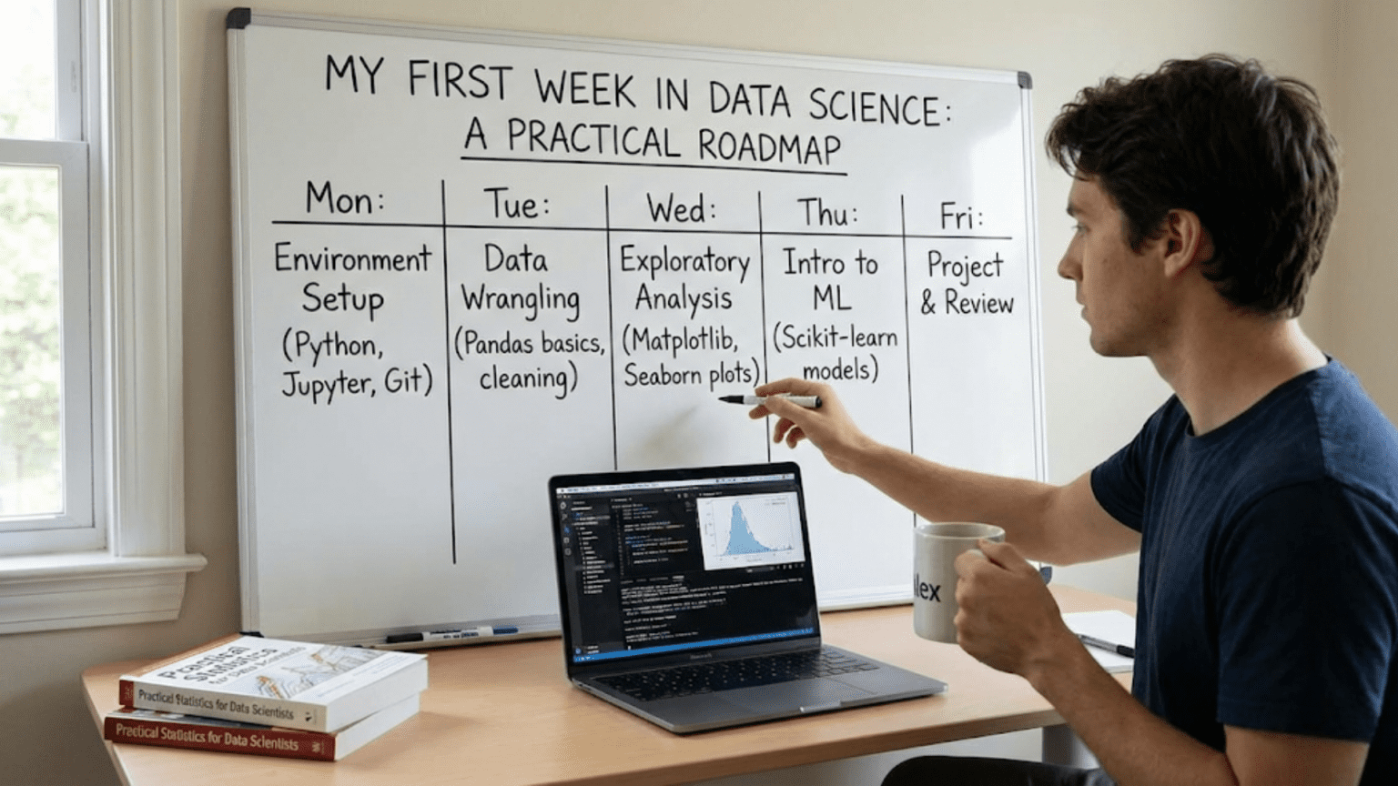
Your first week in data science sets the foundation for everything that follows. Spending this week wisely by focusing on the right fundamentals in the right order creates momentum that carries you forward. This practical roadmap guides you day by day through your first week, telling you exactly what to focus on, what to practice, and what to build. By the end of the week, you will have written real Python code, analyzed actual data, created visualizations, and completed a small but complete data science project. Let me show you how to make this week count.
Day One: Python Basics and Getting Comfortable with Jupyter
Your first day should focus on becoming comfortable with your tools and learning the absolute basics of Python programming. Resist the temptation to jump ahead to data analysis before mastering these fundamentals. Solid basics make everything else easier.
Start by launching Jupyter Notebook following the steps you learned during installation. Open Anaconda Prompt on Windows or Terminal on Mac or Linux, type jupyter notebook, and press Enter. Your browser opens to the Jupyter interface. Navigate to a folder where you want to keep your learning notebooks, perhaps creating a new folder called “learning-data-science.” Create a new notebook and name it something like “day-1-python-basics.ipynb.”
Begin with the classic programming introduction: printing output. In the first cell, type:
print("Hello, Data Science!")Press Shift+Enter to run the cell. Seeing the output appear below confirms everything works. This simple act of writing code and seeing results establishes the basic feedback loop you will use throughout your learning.
Variables are your first substantial Python concept. Variables store data that you can reference and manipulate later. Create variables holding different types of data:
# Numbers
age = 25
height = 5.9
temperature = -2.5

# Text (strings)
name = "Alex"
city = "San Francisco"

# Boolean values
is_student = True
has_experience = False

# Display variables
print(name)
print(age)
print(is_student)Type this code into cells and run them. Notice how Python handles different data types. Try creating your own variables with your actual information. Experimenting with the code builds understanding better than just reading.
Learn about data types and how to check them:
# Check types
print(type(age))
print(type(name))
print(type(is_student))

# Convert between types
age_text = str(age)
print(type(age_text))

height_number = float("6.1")
print(type(height_number))Understanding data types prevents confusion later when operations behave differently for numbers versus text. Spend time experimenting with type conversions to build intuition.
Basic arithmetic operations let you perform calculations:
# Basic math
x = 10
y = 3

addition = x + y
subtraction = x - y
multiplication = x * y
division = x / y
floor_division = x // y
modulo = x % y
exponent = x ** y

print("Addition:", addition)
print("Division:", division)
print("Floor division:", floor_division)
print("Modulo:", modulo)Work through these examples, changing the numbers to see how results change. Understanding these operations now prepares you for mathematical operations on data later.
String manipulation skills help you work with text data:
# String operations
first_name = "John"
last_name = "Smith"

# Concatenation
full_name = first_name + " " + last_name
print(full_name)

# String methods
print(full_name.upper())
print(full_name.lower())
print(full_name.replace("Smith", "Doe"))

# String formatting
age = 30
message = f"{first_name} is {age} years old"
print(message)Practice these operations with different strings. String manipulation is fundamental for working with text data in real datasets.
End your first day by practicing with lists, Python’s most basic data structure:
# Creating lists
numbers = [1, 2, 3, 4, 5]
names = ["Alice", "Bob", "Charlie"]
mixed = [1, "hello", True, 3.14]

# Accessing elements
print(numbers[0])  # First element
print(numbers[-1])  # Last element

# Adding elements
numbers.append(6)
print(numbers)

# List length
print(len(numbers))Lists will be everywhere in your data science work. Getting comfortable with creating and accessing list elements establishes important foundations.
By the end of day one, you should feel comfortable launching Jupyter, creating notebooks, running code cells, and working with basic Python variables, operations, and lists. Do not worry about memorizing everything. Focus on understanding the concepts and knowing you can return to your notebook to reference examples. Spend three to four hours on this material, ensuring you type and run all examples yourself rather than just reading.
Day Two: Control Flow and Functions
Day two builds on yesterday’s basics by introducing control flow that lets programs make decisions and repeat operations, plus functions that organize code into reusable blocks. These concepts transform simple programs into powerful tools.
Start with conditional statements that let programs make decisions based on conditions:
# If statements
temperature = 75

if temperature > 80:
    print("It's hot!")
elif temperature > 60:
    print("It's comfortable")
else:
    print("It's cold!")

# Comparison operators
age = 25
print(age > 18)  # True
print(age == 30)  # False
print(age != 25) # FalsePractice writing conditional statements with different scenarios. Try creating a program that categorizes ages into child, teenager, adult, and senior based on different thresholds.
Loops let you repeat operations multiple times without writing repetitive code:
# For loops
numbers = [1, 2, 3, 4, 5]

for num in numbers:
    print(num * 2)

# Range function
for i in range(5):
    print(f"Count: {i}")

# While loops
count = 0
while count < 5:
    print(count)
count += 1Loops are fundamental for data processing where you need to perform the same operation on many data points. Practice creating loops that process different lists and ranges.
Functions organize code into named blocks you can reuse:
# Defining functions
def greet(name):
    return f"Hello, {name}!"

# Calling functions
message = greet("Alice")
print(message)

# Functions with multiple parameters
def calculate_area(length, width):
    area = length * width
    return area

room_area = calculate_area(10, 15)
print(f"Room area: {room_area}")

# Functions with default parameters
def introduce(name, age=30):
    return f"{name} is {age} years old"

print(introduce("Bob"))
print(introduce("Carol", 25))Write several functions yourself. Try creating a function that converts Celsius to Fahrenheit, another that calculates the average of a list of numbers, and one that checks if a number is even or odd.
Combine concepts by writing small programs that use conditionals, loops, and functions together:
# Program that processes a list of temperatures
def categorize_temperature(temp):
    if temp > 80:
        return "hot"
    elif temp > 60:
        return "comfortable"
    else:
        return "cold"

temperatures = [75, 62, 85, 55, 90, 68]

for temp in temperatures:
    category = categorize_temperature(temp)
    print(f"{temp}°F is {category}")

# Program that finds even numbers
def is_even(number):
    return number % 2 == 0

numbers = range(1, 11)
even_numbers = []

for num in numbers:
    if is_even(num):
        even_numbers.append(num)

print("Even numbers:", even_numbers)These combined examples show how basic programming concepts work together to solve problems. Spend time creating your own programs that combine multiple concepts.
Practice exercises solidify your understanding. Try these challenges:
- Write a function that takes a list of numbers and returns only the ones greater than 10
- Create a program that counts how many vowels are in a string
- Write a function that takes a temperature and unit (C or F) and converts it to the other unit
- Create a program that generates a list of the first 10 square numbers
Do not move on until you can complete at least two of these exercises. Actually writing code builds skills far more effectively than reading about code. Expect to spend four to five hours on day two material, with substantial time devoted to practice exercises.
Day Three: Introduction to NumPy and Arrays
Day three introduces your first data science library. NumPy provides powerful tools for numerical computing that form the foundation of most data science work in Python. Understanding NumPy arrays prepares you for pandas DataFrames tomorrow.
Import NumPy in a new notebook:
import numpy as np

# Create arrays
arr1 = np.array([1, 2, 3, 4, 5])
print(arr1)
print(type(arr1))

# Array from range
arr2 = np.arange(0, 10, 2)  # Start, stop, step
print(arr2)

# Arrays of zeros and ones
zeros = np.zeros(5)
ones = np.ones(5)
print(zeros)
print(ones)NumPy arrays look similar to Python lists but offer much more functionality for numerical operations. Experiment with creating arrays using different methods.
Array operations demonstrate NumPy’s power:
# Vectorized operations (no loops needed!)
arr = np.array([1, 2, 3, 4, 5])

# All elements multiplied by 2
doubled = arr * 2
print(doubled)

# All elements squared
squared = arr ** 2
print(squared)

# Operations between arrays
arr1 = np.array([1, 2, 3])
arr2 = np.array([4, 5, 6])
combined = arr1 + arr2
print(combined)This vectorized operation style is fundamental to efficient data science code. Operations apply to entire arrays without explicit loops, making code both clearer and faster.
Learn to access array elements:
arr = np.array([10, 20, 30, 40, 50])

# Indexing
print(arr[0])   # First element
print(arr[-1])  # Last element
print(arr[1:4]) # Slicing

# Boolean indexing
print(arr > 25)  # Returns boolean array
print(arr[arr > 25]) # Returns elements where condition is TrueBoolean indexing becomes crucial for filtering data later. Practice creating different conditions and filtering arrays.
Explore array statistics:
data = np.array([23, 45, 67, 12, 89, 34, 56])

# Common statistics
print("Mean:", np.mean(data))
print("Median:", np.median(data))
print("Standard deviation:", np.std(data))
print("Min:", np.min(data))
print("Max:", np.max(data))
print("Sum:", np.sum(data))These statistical functions will be used constantly in data analysis. Understanding what each measures helps you describe and understand datasets.
Work with multidimensional arrays:
# 2D arrays (like spreadsheets)
arr_2d = np.array([[1, 2, 3],
                   [4, 5, 6],
                   [7, 8, 9]])

print(arr_2d)
print("Shape:", arr_2d.shape)  # Dimensions

# Accessing 2D arrays
print(arr_2d[0, 0])  # First row, first column
print(arr_2d[1, :])  # Second row, all columns
print(arr_2d[:, 1]) # All rows, second columnTwo-dimensional arrays represent tabular data, preparing you for working with datasets that have rows and columns.
Generate random data for practice:
# Random numbers
random_data = np.random.randint(1, 100, 20)  # 20 random integers
print(random_data)
print("Mean of random data:", np.mean(random_data))

# Normal distribution
normal_data = np.random.normal(50, 10, 1000)  # Mean 50, std 10
print("Mean:", np.mean(normal_data))
print("Std:", np.std(normal_data))Generating random data helps you practice operations and later lets you create test datasets for learning algorithms.
Complete these practice exercises:
- Create an array of numbers from 1 to 100 and find all numbers divisible by 7
- Generate random test scores for 30 students and calculate the class average
- Create a 5×5 multiplication table using NumPy arrays
- Given an array of temperatures in Fahrenheit, convert all to Celsius
Spend four to five hours on NumPy, ensuring you understand array operations deeply. NumPy thinking (operating on entire arrays rather than looping through elements) is a mindset shift that pays enormous dividends later.
Day Four: Pandas for Data Manipulation
Day four introduces pandas, the library you will use most frequently for data analysis. Pandas DataFrames represent tabular data similar to spreadsheets, providing powerful tools for loading, cleaning, and analyzing data.
Import pandas and create your first DataFrame:
import pandas as pd

# Create DataFrame from dictionary
data = {
    'name': ['Alice', 'Bob', 'Charlie', 'David', 'Eve'],
    'age': [25, 30, 35, 28, 32],
    'city': ['NYC', 'LA', 'Chicago', 'Houston', 'Phoenix'],
    'salary': [70000, 80000, 75000, 72000, 85000]
}

df = pd.DataFrame(data)
print(df)A DataFrame organizes data into rows and columns with labels, making it easy to work with structured information. This is the data structure you will use for almost all data analysis.
Explore DataFrame basics:
# View first few rows
print(df.head())

# View last few rows
print(df.tail())

# DataFrame information
print(df.info())

# Summary statistics
print(df.describe())

# Access columns
print(df['name'])
print(df.age)  # Alternative syntax

# Access rows by position
print(df.iloc[0])  # First row

# Access rows by condition
print(df[df['age'] > 30])Practice each of these operations to understand how to examine and access data in DataFrames. These techniques will be used in every analysis you do.
Load data from files:
# Create sample CSV file first
df.to_csv('sample_data.csv', index=False)

# Read CSV file
df_loaded = pd.read_csv('sample_data.csv')
print(df_loaded)

# Read Excel (if you have openpyxl installed)
# df.to_excel('sample_data.xlsx', index=False)
# df_excel = pd.read_excel('sample_data.xlsx')Loading data from files is how real data science projects begin. Understanding file operations prepares you for working with actual datasets.
Filter and select data:
# Select specific columns
names_and_ages = df[['name', 'age']]
print(names_and_ages)

# Filter rows
high_earners = df[df['salary'] > 75000]
print(high_earners)

# Multiple conditions
young_high_earners = df[(df['age'] < 30) & (df['salary'] > 70000)]
print(young_high_earners)Filtering data to find subsets meeting specific criteria is fundamental to analysis. Practice creating different filter conditions.
Modify and add data:
# Add new column
df['bonus'] = df['salary'] * 0.1
print(df)

# Modify existing column
df['age'] = df['age'] + 1  # Everyone ages a year
print(df)

# Drop columns
df_without_bonus = df.drop('bonus', axis=1)
print(df_without_bonus)Real data analysis often involves creating new columns derived from existing ones. These operations transform data into forms useful for analysis.
Group and aggregate data:
# Group by city and calculate mean salary
city_salaries = df.groupby('city')['salary'].mean()
print(city_salaries)

# Multiple aggregations
stats_by_city = df.groupby('city').agg({
    'salary': ['mean', 'max'],
    'age': 'mean'
})
print(stats_by_city)Grouping data to calculate statistics for different categories is extremely common. Understanding groupby operations enables sophisticated analysis.
Handle missing data:
# Create data with missing values
data_missing = {
    'A': [1, 2, None, 4],
    'B': [5, None, 7, 8],
    'C': [9, 10, 11, 12]
}
df_missing = pd.DataFrame(data_missing)

# Check for missing values
print(df_missing.isnull())
print(df_missing.isnull().sum())

# Drop rows with missing values
print(df_missing.dropna())

# Fill missing values
print(df_missing.fillna(0))
print(df_missing.fillna(df_missing.mean()))Real datasets always have missing values. Knowing how to detect and handle them is essential.
Complete these exercises:
- Create a DataFrame with information about 10 books (title, author, year, rating)
- Filter to find books published after 2010 with ratings above 4
- Add a column calculating how many years old each book is
- Group by author and find the average rating of their books
Pandas is vast, but these fundamentals enable you to start analyzing real data. Spend four to five hours practicing pandas operations until they feel natural.
Day Five: Data Visualization with Matplotlib
Day five focuses on creating visualizations that help you understand data and communicate findings. Matplotlib provides the foundation for plotting in Python.
Start with basic line plots:
import matplotlib.pyplot as plt
import numpy as np

# Create data
x = np.arange(0, 10, 0.1)
y = np.sin(x)

# Create plot
plt.figure(figsize=(10, 6))
plt.plot(x, y)
plt.title('Sine Wave')
plt.xlabel('X values')
plt.ylabel('Y values')
plt.grid(True)
plt.show()Creating this first plot demonstrates the complete plotting workflow: creating data, setting up the figure, plotting data, adding labels, and displaying the result.
Explore different plot types:
import pandas as pd

# Create sample data
data = {
    'category': ['A', 'B', 'C', 'D', 'E'],
    'values': [23, 45, 56, 78, 32]
}
df = pd.DataFrame(data)

# Bar chart
plt.figure(figsize=(10, 6))
plt.bar(df['category'], df['values'])
plt.title('Bar Chart Example')
plt.xlabel('Category')
plt.ylabel('Values')
plt.show()

# Scatter plot
x = np.random.randn(100)
y = 2 * x + np.random.randn(100) * 0.5

plt.figure(figsize=(10, 6))
plt.scatter(x, y, alpha=0.5)
plt.title('Scatter Plot Example')
plt.xlabel('X')
plt.ylabel('Y')
plt.show()

# Histogram
data = np.random.normal(100, 15, 1000)

plt.figure(figsize=(10, 6))
plt.hist(data, bins=30, edgecolor='black')
plt.title('Histogram Example')
plt.xlabel('Value')
plt.ylabel('Frequency')
plt.show()Different plot types reveal different aspects of data. Bar charts compare categories, scatter plots show relationships, and histograms display distributions.
Customize plot appearance:
# Multiple lines on one plot
x = np.linspace(0, 10, 100)
y1 = np.sin(x)
y2 = np.cos(x)

plt.figure(figsize=(12, 6))
plt.plot(x, y1, label='sin(x)', color='blue', linewidth=2)
plt.plot(x, y2, label='cos(x)', color='red', linewidth=2, linestyle='--')
plt.title('Sine and Cosine', fontsize=16)
plt.xlabel('X', fontsize=12)
plt.ylabel('Y', fontsize=12)
plt.legend()
plt.grid(True, alpha=0.3)
plt.show()Customization makes plots clearer and more professional. Experiment with colors, line styles, and formatting options.
Create subplots to show multiple visualizations:
# Create 2x2 grid of plots
fig, axes = plt.subplots(2, 2, figsize=(12, 10))

# Plot in each subplot
axes[0, 0].plot([1, 2, 3, 4], [1, 4, 2, 3])
axes[0, 0].set_title('Line Plot')

axes[0, 1].scatter([1, 2, 3, 4], [1, 4, 2, 3])
axes[0, 1].set_title('Scatter Plot')

axes[1, 0].bar(['A', 'B', 'C'], [10, 20, 15])
axes[1, 0].set_title('Bar Chart')

axes[1, 1].hist(np.random.randn(1000), bins=30)
axes[1, 1].set_title('Histogram')

plt.tight_layout()
plt.show()Subplots let you compare multiple visualizations side by side, making patterns across different views of the data easier to spot.
Practice exercises:
- Create a line plot showing your city’s average temperature by month (make up data)
- Generate 100 random points and create a scatter plot colored by whether they are above or below y=0
- Create a bar chart comparing sales for different products
- Make a histogram showing the distribution of exam scores for a class
Spend three to four hours creating various visualizations. Visualization skills grow through practice and experimentation. Do not worry about making perfect plots yet; focus on understanding how to create different chart types.
Day Six: Your First Data Analysis Project
Day six brings everything together in a complete data analysis project. You will load real data, clean it, analyze it, and create visualizations to answer questions. This integrated practice solidifies the skills you have learned.
For this project, use a simple dataset about sales or students or any topic that interests you. You can create synthetic data or download a beginner-friendly dataset from sources like Kaggle. Here is an example creating synthetic sales data:
import pandas as pd
import numpy as np
import matplotlib.pyplot as plt

# Create synthetic sales data
np.random.seed(42)

dates = pd.date_range('2024-01-01', periods=100)
products = np.random.choice(['Product A', 'Product B', 'Product C'], 100)
quantities = np.random.randint(1, 20, 100)
prices = np.random.choice([10.99, 15.99, 12.99], 100)
sales = quantities * prices

df = pd.DataFrame({
    'date': dates,
    'product': products,
    'quantity': quantities,
    'price': prices,
    'total_sale': sales
})

# Save to CSV
df.to_csv('sales_data.csv', index=False)
print("Data created and saved")
print(df.head())Now analyze this data step by step:
# Load data
df = pd.read_csv('sales_data.csv')
df['date'] = pd.to_datetime(df['date'])

# 1. Basic exploration
print("Dataset shape:", df.shape)
print("\nFirst few rows:")
print(df.head())

print("\nDataset info:")
print(df.info())

print("\nSummary statistics:")
print(df.describe())

# 2. Answer specific questions
print("\nTotal sales:", df['total_sale'].sum())
print("Average sale amount:", df['total_sale'].mean())
print("Number of transactions:", len(df))

# 3. Sales by product
sales_by_product = df.groupby('product')['total_sale'].sum()
print("\nSales by product:")
print(sales_by_product)

# 4. Best selling product by quantity
quantity_by_product = df.groupby('product')['quantity'].sum()
print("\nQuantity sold by product:")
print(quantity_by_product)

# 5. Create visualizations
# Sales by product - bar chart
plt.figure(figsize=(10, 6))
sales_by_product.plot(kind='bar')
plt.title('Total Sales by Product')
plt.xlabel('Product')
plt.ylabel('Total Sales ($)')
plt.xticks(rotation=45)
plt.tight_layout()
plt.savefig('sales_by_product.png')
plt.show()

# Daily sales trend - line plot
df['date'] = pd.to_datetime(df['date'])
daily_sales = df.groupby('date')['total_sale'].sum()

plt.figure(figsize=(12, 6))
plt.plot(daily_sales.index, daily_sales.values)
plt.title('Daily Sales Trend')
plt.xlabel('Date')
plt.ylabel('Total Sales ($)')
plt.xticks(rotation=45)
plt.grid(True, alpha=0.3)
plt.tight_layout()
plt.savefig('daily_sales_trend.png')
plt.show()

# Distribution of sale amounts - histogram
plt.figure(figsize=(10, 6))
plt.hist(df['total_sale'], bins=20, edgecolor='black')
plt.title('Distribution of Sale Amounts')
plt.xlabel('Sale Amount ($)')
plt.ylabel('Frequency')
plt.tight_layout()
plt.savefig('sale_distribution.png')
plt.show()Document your analysis with markdown cells explaining what each section does and what you discovered. This practice of documenting analysis is crucial for real work.
Challenge yourself to answer additional questions:
- Which day had the highest total sales?
- What is the average quantity purchased per transaction for each product?
- Are there any unusual patterns or outliers in the data?
- What recommendations would you make based on this analysis?
Create a complete notebook that tells a story: introduce the data, ask questions, analyze to find answers, create visualizations, and state conclusions. This structure mirrors real data science work.
Spend five to six hours on this project. The goal is not perfection but completion. Finishing an entire analysis from start to finish, even a simple one, builds confidence and demonstrates that you can do data science.
Day Seven: Review, Practice, and Plan Ahead
Your final day of week one should consolidate learning, fill gaps, and set direction for continued growth. Do not introduce completely new concepts; instead, reinforce what you have learned.
Review your notebooks from the week:
- Day 1: Python basics
- Day 2: Control flow and functions
- Day 3: NumPy arrays
- Day 4: Pandas DataFrames
- Day 5: Matplotlib visualization
- Day 6: Complete analysis project
Identify concepts that still feel unclear. Revisit those sections and work through examples again. Understanding builds through repetition and practice.
Complete additional practice exercises combining multiple skills:
Exercise 1: Temperature Analysis
- Create a dataset with daily temperatures for a month
- Calculate weekly averages
- Identify the hottest and coldest days
- Plot temperature trends
- Create a histogram showing temperature distribution
Exercise 2: Student Grade Analysis
- Create a dataset with student names, scores on three tests, and homework grades
- Calculate each student’s average grade
- Determine letter grades based on averages
- Find the class average for each assessment
- Create visualizations showing grade distributions
- Identify students who need extra help (below certain threshold)
Exercise 3: Product Inventory
- Create a dataset with product names, quantities in stock, prices, and categories
- Calculate total inventory value
- Identify low-stock items (below 5 units)
- Find the most expensive items
- Calculate average price by category
- Create visualizations showing inventory by category
Work through at least two of these exercises completely, creating clean notebooks with explanations. Each exercise requires combining Python basics, pandas operations, and visualization skills.
Reflect on your progress by answering these questions:
- What concepts do I understand well?
- What topics need more practice?
- What surprised me this week?
- What did I find most challenging?
- What did I enjoy most?
Write your reflections in a markdown cell. This metacognition helps you learn more effectively.
Plan your second week:
- Continue practicing pandas with more complex datasets
- Learn about data cleaning and handling messy real-world data
- Explore seaborn for more advanced statistical visualizations
- Start learning basic statistics concepts
- Work on a slightly larger analysis project
Set specific goals for next week. Vague intentions like “learn more” are less effective than concrete goals like “complete three data analysis projects” or “learn to handle missing data in datasets.”
Consider joining a data science community:
- Reddit’s r/learnpython and r/datascience
- Stack Overflow for asking questions
- Local data science meetups
- Online Discord servers for data science learners
Community provides support, answers questions, and exposes you to how others approach problems.
What You Have Accomplished in One Week
Look back at where you started seven days ago. You knew little or no Python. Data science seemed mysterious and complex. Now you can write Python code confidently, manipulate data with pandas, create visualizations, and complete basic data analysis projects. This represents substantial progress in just one week.
You have learned Python fundamentals including variables, data types, conditionals, loops, and functions. These building blocks enable you to write programs that solve problems. You can read and understand basic Python code, and more importantly, write your own.
You have explored NumPy for numerical computing, understanding arrays and vectorized operations that form the foundation of efficient data processing. You have mastered pandas basics including creating DataFrames, loading data from files, filtering rows, selecting columns, grouping data, and calculating statistics.
You have created visualizations with matplotlib including line plots, bar charts, scatter plots, and histograms. You can customize plots with titles, labels, colors, and styles. You understand that different plot types reveal different aspects of data.
Most importantly, you have completed an entire data analysis project from beginning to end. You loaded data, explored it, asked questions, analyzed to find answers, created visualizations, and drew conclusions. This end-to-end experience is what data science actually involves.
Conclusion
Your first week in data science laid a solid foundation for continued learning. By focusing on fundamentals and practicing consistently, you have built skills that enable more advanced topics. The key to your success was not trying to learn everything at once but rather progressing systematically through essential concepts.
Data science is learned through doing, not just reading or watching. You spent this week writing code, analyzing data, and creating visualizations. This hands-on practice built real skills that abstract learning cannot provide. Continue this pattern of learning concepts then immediately practicing them in code.
The momentum you have built this week will carry you forward if you maintain consistent practice. Data science mastery comes through accumulating small gains over time, not sudden breakthroughs. Keep showing up, keep practicing, and keep building projects. Each week you will be noticeably better than the week before.
In the next article, we will explore understanding data types in depth, learning about numerical versus categorical data, structured versus unstructured data, and how data types influence what analyses are possible. This knowledge will make you more effective at working with any dataset you encounter.
Key Takeaways
Your first week should progress systematically through fundamentals rather than jumping to advanced topics, starting with Python basics, control flow, and functions before introducing data science libraries. Day one covers variables and basic operations, day two adds conditionals and loops, establishing programming foundations that support everything else.
Days three and four introduce NumPy arrays and pandas DataFrames, the core data structures for numerical computing and data analysis respectively. Understanding array operations and DataFrame manipulation enables you to load, clean, filter, group, and analyze data effectively.
Day five focuses on matplotlib visualization, teaching you to create line plots, bar charts, scatter plots, and histograms that help you understand data and communicate findings. Different plot types reveal different aspects of data, and customization makes visualizations clearer and more professional.
Day six brings everything together in a complete data analysis project where you load data, explore it, answer questions through analysis, create visualizations, and draw conclusions. This integrated practice demonstrates that you can actually do data science, not just learn isolated concepts.
Day seven consolidates learning through review and additional practice, helping you identify gaps in understanding and setting direction for continued growth. Consistent daily practice throughout the week builds momentum that carries you forward, with each concept building naturally on previous ones to create a solid foundation for advanced topics.