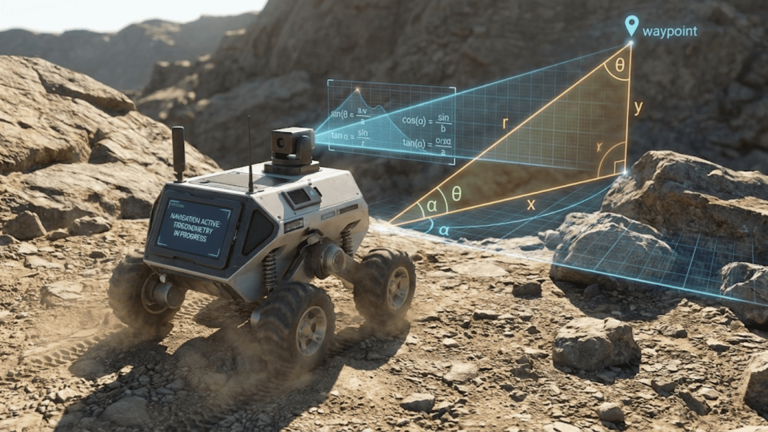
Many people who struggled with trigonometry in school wonder whether they will ever actually use sine, cosine, and tangent functions in real life. If you pursue robotics, the answer becomes an emphatic yes—trigonometry proves indispensable for robots that navigate through space, orient themselves toward targets, or calculate positions from sensor readings. Yet the trigonometry robots need differs substantially from memorizing identities and solving arbitrary triangles in math class. Robot trigonometry serves concrete purposes: calculating how to reach a destination, determining where the robot is based on what sensors see, and converting between different ways of describing positions and orientations.

The connection between trigonometry and robot navigation becomes obvious once you recognize that navigation fundamentally involves triangles. When your robot detects an object at a certain angle and distance, those measurements form a triangle connecting the robot, the object, and the coordinate axes. When your robot needs to turn toward a target, calculating the required angle involves triangle geometry. When sensors measure angles and your robot needs distances, or vice versa, trigonometric functions convert between these quantities. Rather than abstract mathematical exercises, robot trigonometry solves practical geometric problems that robots encounter constantly.

This article explains why trigonometry matters for robot navigation by exploring specific problems robots face and showing how trigonometric functions solve them. You will learn what sine, cosine, and tangent actually measure in physical terms, how robots use these functions for navigation tasks, and how to think about trigonometry geometrically rather than as abstract formulas. By understanding trigonometry through robotics applications, even the most trigonometry-averse readers will appreciate these functions as practical tools rather than academic torture devices.

What Sine, Cosine, and Tangent Actually Measure

Before examining robot applications, clarifying what trigonometric functions actually represent helps you understand why robots use them. These functions describe relationships in right triangles—triangles with one 90-degree angle.

Consider a right triangle with one angle (besides the right angle) marked as θ (theta). The three sides have names relative to this angle: the hypotenuse is the longest side opposite the right angle, the opposite side is the side across from angle θ, and the adjacent side is the side next to angle θ (not the hypotenuse). These relative labels depend on which angle you are considering.

Sine of angle θ equals the ratio of the opposite side length to the hypotenuse length: sin(θ) = opposite/hypotenuse. If the opposite side measures 3 units and hypotenuse measures 5 units, then sin(θ) = 3/5 = 0.6. This ratio remains constant for any right triangle with the same angle θ, regardless of the triangle’s absolute size. Doubling all side lengths doubles both numerator and denominator, leaving the ratio unchanged. This scale-independence makes sine useful—knowing the angle tells you the ratio, or knowing the ratio tells you the angle.

Cosine of angle θ equals the ratio of the adjacent side to the hypotenuse: cos(θ) = adjacent/hypotenuse. Using the classic 3-4-5 right triangle with angle θ opposite the side of length 3, the adjacent side measures 4 units, so cos(θ) = 4/5 = 0.8. Cosine provides complementary information to sine—together, sine and cosine completely characterize the angle’s effect on triangle proportions.

Tangent of angle θ equals the ratio of the opposite side to the adjacent side: tan(θ) = opposite/adjacent. For our 3-4-5 triangle, tan(θ) = 3/4 = 0.75. Alternatively, tangent equals sine divided by cosine: tan(θ) = sin(θ)/cos(θ). This relationship shows that tangent captures the relative proportion of the two legs of the right triangle, independent of hypotenuse length. When the opposite side equals the adjacent side (45-degree angle), tangent equals one. When the opposite side is longer, tangent exceeds one. When adjacent is longer, tangent is less than one.

Inverse trigonometric functions (arcsin, arccos, arctan) reverse these operations, finding angles from ratios. If you know sin(θ) = 0.6, then θ = arcsin(0.6) ≈ 36.87 degrees. These inverse functions enable robots to calculate angles from measurements or computed ratios. When your robot measures two sides of a triangle and needs to know the angle, inverse trigonometric functions provide the answer.

The geometric interpretation helps more than memorized formulas. Sine measures the vertical component of a unit vector at angle θ from horizontal. Cosine measures the horizontal component. If you walk along a line at angle θ, sine tells you how much altitude you gain per unit distance, and cosine tells you how much horizontal distance you cover. This component interpretation appears constantly in robot navigation.

Converting Between Cartesian and Polar Coordinates

Robots often need to convert between two fundamental ways of describing positions: Cartesian coordinates (x, y) specifying horizontal and vertical distances from origin, and polar coordinates (r, θ) specifying distance and angle from origin. Trigonometry provides the conversion formulas.

From polar to Cartesian conversion uses sine and cosine directly. If you know a point sits at distance r and angle θ from origin, its Cartesian coordinates are:

• x = r × cos(θ)
• y = r × sin(θ)

This conversion makes geometric sense: cosine gives the horizontal component and sine gives the vertical component of the position vector. For example, a point at distance 5 and angle 37 degrees has coordinates x = 5×cos(37°) ≈ 4 and y = 5×sin(37°) ≈ 3. These formulas encode how to project the diagonal position vector onto the coordinate axes.

From Cartesian to polar conversion uses inverse trigonometric functions and the Pythagorean theorem. Given Cartesian coordinates (x, y):

• r = √(x² + y²)
• θ = arctan(y/x)

The distance formula uses the Pythagorean theorem—the position vector is the hypotenuse of a right triangle with legs x and y. The angle uses arctan because tangent equals opposite over adjacent, which in this context is y/x. A point at (4, 3) has distance r = √(16+9) = 5 and angle θ = arctan(3/4) ≈ 37 degrees.

The arctan conversion requires care about angle quadrants. Simple arctan returns angles between -90 and +90 degrees, which cannot distinguish between all four quadrants. The two-argument form atan2(y, x) available in most programming languages correctly handles all quadrants, returning angles from -180 to +180 degrees (or 0 to 360 depending on convention). Always use atan2 when converting from Cartesian to polar coordinates to avoid quadrant ambiguity.

Why robots need both coordinate systems becomes clear in different contexts. Sensors often provide polar data—distance sensors measure r and angular position of a target provides θ. However, obstacle maps and path planning naturally work in Cartesian coordinates. Converting sensor readings from polar to Cartesian lets robots build Cartesian maps. Conversely, if you know target position in Cartesian coordinates and need to determine heading, converting to polar gives the angle directly.

These conversions appear constantly in navigation code. A robot planning path to Cartesian position (10, 5) from origin first converts to polar, finding it needs to point toward angle arctan(5/10) ≈ 27 degrees. Once oriented, it travels distance √(10² + 5²) ≈ 11.2 units. This example shows how Cartesian goals convert to polar navigation commands naturally through trigonometry.

Calculating Heading Angles Toward Targets

One of the most common navigation problems is determining what angle to turn toward a target position. Trigonometry provides straightforward solution through the angle calculation we just discussed, but understanding the full context helps.

Given robot at position (x_robot, y_robot) and target at (x_target, y_target), the angle from robot to target relative to the X-axis is:

• Δx = x_target – x_robot
• Δy = y_target – y_robot
• θ = atan2(Δy, Δx)

This calculation finds the displacement vector from robot to target, then calculates its angle. For example, if robot sits at (2, 1) and target at (7, 4), displacement is (5, 3) and angle is atan2(3, 5) ≈ 31 degrees from the X-axis. This tells the robot which direction points toward the target.

However, robots typically need to know how much to turn from their current heading, not the absolute angle. If the robot currently faces 45 degrees and the target angle is 31 degrees, the robot should turn -14 degrees (turn right 14 degrees). The required turn angle equals target angle minus current heading:

• turn_angle = θ_target – θ_current

Handling angle wraparound complicates this subtraction. If current heading is 350 degrees and target is 10 degrees, naive subtraction gives 10 – 350 = -340 degrees, suggesting a large left turn when actually turning right 20 degrees is correct. Wrapping the difference to the range -180 to +180 degrees fixes this:

turn_angle = (θ_target - θ_current + 180) mod 360 - 180

This wraparound handling ensures the turn angle represents the smallest rotation reaching the target heading.

Robots with differential drive or car-like steering use these heading calculations constantly. The turn angle determines motor commands—positive angles command left turns, negative angles command right turns. The magnitude determines how much to turn. Once turned, the robot moves forward toward the target. This turn-and-move strategy, repeated iteratively, enables simple navigation toward targets.

More sophisticated navigation might calculate smooth curved paths rather than sharp turns, but even curved path planning uses trigonometry to determine tangent directions at each point along the curve. The heading calculations form building blocks for any navigation approach requiring directional awareness.

Distance and Bearing from Sensor Readings

Many robot sensors provide polar information—angles and distances to detected objects. Trigonometry converts these measurements into Cartesian positions suitable for mapping and obstacle avoidance.

Ultrasonic or infrared distance sensors typically mount at fixed positions on the robot with known orientations. If a sensor points at angle α relative to the robot’s heading and measures distance d to an obstacle, the obstacle’s position in robot body frame is:

• x_obstacle = d × cos(α)
• y_obstacle = d × sin(α)

This calculation transforms the polar sensor reading (d, α) into Cartesian coordinates relative to the robot. For example, a sensor pointing 30 degrees to the right measuring distance 2 meters places the obstacle at x = 2×cos(-30°) ≈ 1.73 meters forward and y = 2×sin(-30°) ≈ -1 meter to the right (negative y meaning right).

LIDAR sensors sweep through angular range, measuring distances at many angles. Each LIDAR reading provides distance d_i at angle α_i, converting to Cartesian point cloud:

• x_i = d_i × cos(α_i)
• y_i = d_i × sin(α_i)

Processing LIDAR data to build obstacle maps relies on these trigonometric conversions. The point cloud in robot body frame can then transform to world frame using the robot’s position and orientation, building a consistent map as the robot moves.

Bearing-only sensors that detect angles to targets without measuring distances present different challenge. If you observe a landmark at angle θ from two different robot positions, triangulation uses these angles to calculate landmark position. The mathematics involves solving triangle formed by the two robot positions and the landmark using angle measurements and known distance between observation positions. This triangulation fundamentally uses trigonometry to infer distances from angles.

Acoustic or radio direction-finding that measures signal direction but not distance similarly requires trigonometry for position calculation. Multiple direction measurements from different locations enable triangulation computing source position. The geometric relationships solving these problems all reduce to trigonometry on triangles formed by measurement positions and target locations.

Robot Arm Kinematics and Joint Angles

Robot manipulators provide even clearer trigonometry applications because joint angles directly determine end-effector positions through trigonometric relationships.

For a simple two-joint planar arm, forward kinematics calculates end-effector position from joint angles using trigonometry explicitly. If the first link has length L1 and rotates by angle θ1, its tip reaches position:

• x1 = L1 × cos(θ1)
• y1 = L1 × sin(θ1)

Adding the second link of length L2 at angle θ2 relative to the first link, the end-effector position becomes:

• x = L1×cos(θ1) + L2×cos(θ1 + θ2)
• y = L1×sin(θ1) + L2×sin(θ1 + θ2)

These formulas chain the effects of each joint’s rotation, with each joint contributing horizontal and vertical components determined by sine and cosine of its angle. This trigonometric formulation extends to any number of joints, though the formulas grow longer.

Inverse kinematics for the two-joint arm solves for joint angles given desired end-effector position. The geometric solution involves finding angles of a triangle formed by the two links and the distance to the target. Using the law of cosines to find the elbow angle θ2:

• cos(θ2) = (x² + y² – L1² – L2²) / (2×L1×L2)
• θ2 = arccos(above)

Then solving for base angle θ1 using trigonometry on the triangle formed by the base, the target, and the second link. The full derivation involves substantial trigonometry, but the point is that inverse kinematics fundamentally requires trigonometric calculations to relate joint angles to spatial positions.

More complex arms use more sophisticated mathematics, but trigonometry remains central. Three-dimensional arms use three-dimensional trigonometry with sine and cosine in multiple planes. Robot arm control software performs these trigonometric calculations thousands of times per second, continuously computing forward and inverse kinematics as the arm moves.

The trigonometry in kinematics seems abstract when written as formulas, but visualizing it geometrically makes sense. Each joint rotates a link by some angle, projecting the link’s length onto horizontal and vertical directions according to sine and cosine of the rotation angle. Chaining these projections through multiple joints gives the overall effect. This geometric picture transforms trigonometric formulas from mysterious symbols into sensible calculations describing how joint rotations create end-effector motion.

Odometry and Tracking Robot Position

Mobile robots estimate their position through odometry—integrating wheel rotations over time to track cumulative motion. This dead reckoning navigation fundamentally depends on trigonometry to update position based on motion measurements.

For differential drive robots (two independently driven wheels), the measured wheel rotations determine how far each wheel traveled. If the left wheel travels distance d_left and right wheel travels d_right, the robot rotates by angle:

• Δθ = (d_right – d_left) / w

where w is the wheelbase (distance between wheels). This rotation calculation comes from the geometry of how differential motion creates turning—one wheel traveling farther than the other causes rotation around a point between the wheels.

The distance the robot’s center travels is:

• d = (d_left + d_right) / 2

This average distance represents how far the robot moved forward (or backward if negative).

Updating the robot’s position using these motion measurements requires trigonometry. If the robot starts at position (x, y) with heading θ, after moving distance d and rotating Δθ, the new position is:

• x_new = x + d × cos(θ + Δθ/2)
• y_new = y + d × sin(θ + Δθ/2)
• θ_new = θ + Δθ

The trigonometric terms project the motion distance d along the robot’s heading direction to calculate how much the X and Y coordinates change. Using θ + Δθ/2 (heading at the middle of the motion) provides better accuracy than using initial or final heading alone, accounting for the curved path the robot follows when turning while moving.

This odometry update repeats at high frequency, chaining many small motions to track overall robot path. Each update uses trigonometry to project the incremental motion onto the coordinate axes. While odometry accumulates errors over time (wheel slip, measurement noise), the basic mechanism using trigonometry to integrate motion into position tracking enables all dead reckoning navigation.

Car-like robots with Ackermann steering use similar trigonometry but with different geometric models. The turning radius depends on steering angle, and the motion follows circular arc rather than straight line. Calculating position updates for circular arc motion requires more complex trigonometry, but the fundamental principle remains: use sine and cosine to project motion along the current heading onto coordinate axes.

Path Following and Pure Pursuit Control

When robots follow planned paths, they must continuously adjust heading to stay on track. Pure pursuit is a classic path-following algorithm that uses trigonometry to calculate steering angles.

Pure pursuit picks a look-ahead point some distance ahead on the desired path and steers toward that point. If the look-ahead point sits at distance L from the robot and angle α from the robot’s heading, the required steering curvature is:

• κ = 2×sin(α) / L

This formula comes from the geometry of circular arcs. The robot needs to follow an arc of radius R reaching the look-ahead point, and geometric analysis shows that curvature κ = 1/R relates to angle α through this trigonometric formula. The sine function captures how much lateral deviation (perpendicular to heading) exists compared to forward distance.

For car-like robots, steering angle δ relates to path curvature through:

• δ = arctan(κ × w)

where w is the wheelbase. This conversion from curvature to steering angle again uses inverse trigonometry—specifically arctangent—to translate the geometric curvature requirement into a physical steering angle.

Different path-following algorithms use variations of these ideas, but all depend on trigonometry to calculate heading corrections based on geometric relationships between current robot pose and desired path. Cross-track error (perpendicular distance from path) combines with heading error (angle difference between robot heading and path tangent) through trigonometric functions to determine required steering commands.

Understanding path following through trigonometry clarifies why these algorithms work. The trigonometric calculations compute geometrically optimal steering angles that naturally guide robots toward and along desired paths. Pure pursuit succeeds because its trigonometric formula correctly captures the geometry of circular arc motion that robots actually execute.

Avoiding Trigonometric Pitfalls in Robot Code

While trigonometry enables robot navigation, several common mistakes cause bugs that can be frustrating to debug.

Angle units confusion between degrees and radians causes mysterious scaling errors. Most programming language trigonometric functions expect radians (where 360 degrees equals 2π radians), but humans think in degrees, and some sensors report degrees. Mixing units produces wrong results by factors of roughly 57 (the conversion factor). Always know what units your angles use and convert consistently. Many bugs come from forgetting to convert degrees to radians before calling trigonometric functions, or vice versa.

Angle wraparound at 360 degrees (or 180 or π depending on convention) creates discontinuous jumps in angle values. An angle that increases from 359 to 1 degree jumps discontinuously from 359 to 1 rather than smoothly continuing to 360 ≡ 0. This discontinuity breaks algorithms that compute angle differences or average angles. Proper angle wraparound handling normalizes angles to preferred ranges and handles arithmetic that crosses boundaries. The modulo operation helps, but care is required to handle negative angles correctly.

Arctangent quadrant ambiguity from using atan() instead of atan2() causes angles in wrong quadrants. Standard atan returns angles only from -90 to +90 degrees, but target positions exist in all four quadrants around the robot. Using atan2(y, x) rather than atan(y/x) resolves quadrant correctly because atan2 uses the signs of both arguments to determine quadrant. Never use atan for angle calculations from Cartesian coordinates—always use atan2.

Gimbal lock in three-dimensional rotations creates singularities where small orientation changes require large angle changes. Representing three-dimensional rotations as sequences of rotations around axes (Euler angles) breaks down at certain orientations. While two-dimensional navigation avoids this issue, three-dimensional robot arms or flying robots must handle gimbal lock carefully through quaternions or other rotation representations that avoid singularities.

Numerical precision issues affect trigonometric calculations involving very small or very large angles. Computers represent numbers with finite precision, causing rounding errors. When computing small angle differences or working near singularities, these rounding errors can dominate results. Using double-precision floating point rather than single precision helps, but awareness that numerical issues exist prevents confusion when results seem slightly wrong.

Practical Tips for Robot Trigonometry

Beyond avoiding errors, several practices make working with trigonometry in robotics smoother and more intuitive.

Visualize calculations geometrically before implementing them. Draw the triangles involved. Label sides and angles. Work through an example by hand using simple numbers. This visualization builds intuition about what calculations accomplish and catches conceptual errors before implementation. Geometric pictures often reveal simpler solution approaches than pure algebraic manipulation produces.

Test trigonometric functions with known values. Sin(0) = 0, sin(90°) = 1, cos(0) = 1, cos(90°) = 0, tan(45°) = 1. When implementing navigation code, test with these simple angles to verify functions work as expected. If sin(90°) does not return 1, you probably forgot to convert degrees to radians. These sanity checks catch unit errors and other mistakes immediately.

Use descriptive variable names that indicate units. Name variables angle_degrees or angle_radians rather than just angle. This self-documentation prevents unit confusion and helps readers understand code. When converting units, make conversion explicit in code even if mathematically unnecessary, documenting what unit conversion accomplishes.

Comment trigonometric calculations explaining the geometry. Mathematical formulas look cryptic to readers (including future you). Comments explaining “calculates the angle from robot to target using arctangent” or “projects motion onto coordinate axes using current heading” make code comprehensible. Geometric explanations help much more than just repeating the formula in words.

Prefer library functions over manual implementation. Modern libraries implement trigonometric functions efficiently and accurately. Writing your own sin() or cos() from scratch teaches mathematics but produces slower, less accurate code than library functions. Use NumPy, math library, or robotics-specific libraries that provide well-tested implementations.

Profile code to identify trigonometric bottlenecks if performance matters. While trigonometric functions compute quickly, calling them millions of times per second might cause performance issues. In performance-critical code, consider caching results, using lookup tables, or reducing calculation frequency. However, optimize only after profiling shows trigonometry actually limits performance—premature optimization often wastes effort.

Beyond Basic Trigonometry

Once comfortable with basic sine, cosine, and tangent, several advanced trigonometric concepts become relevant for sophisticated robot navigation.

Law of cosines extends the Pythagorean theorem to non-right triangles: c² = a² + b² – 2ab×cos(C), where C is the angle between sides a and b. Robot arm inverse kinematics uses law of cosines to find joint angles. Sensor triangulation uses it to calculate distances. This law handles general triangles where simpler right-triangle trigonometry does not apply.

Law of sines relates angles and opposite sides in any triangle: a/sin(A) = b/sin(B) = c/sin(C). Combined with law of cosines, these laws solve arbitrary triangles from partial information. When your robot observes angles to landmarks from multiple positions, law of sines helps compute positions from these angle measurements.

Vector dot product relates to cosine through the formula a·b = |a||b|cos(θ), where θ is the angle between vectors. This connection makes cosine fundamental to vector operations. Calculating whether robots are heading toward or away from targets uses this dot product relationship. Checking if detected objects are in front of or behind the robot uses vector dot products that fundamentally depend on cosine.

Trigonometric identities like sin²(θ) + cos²(θ) = 1 or tan(θ) = sin(θ)/cos(θ) sometimes simplify calculations. While memorizing long lists of identities provides little value, recognizing a few key relationships occasionally reveals simpler solution paths. These identities reflect deeper geometric relationships that can clarify complex calculations.

Fourier analysis decomposes periodic signals into sums of sines and cosines. Robot sensor data often contains periodic noise that Fourier analysis can filter. Understanding that any periodic signal represents as sum of sine and cosine waves of different frequencies enables sophisticated signal processing. This application of trigonometry extends far beyond simple triangle solving into frequency domain analysis.

Trigonometry as Navigation Foundation

Trigonometry might have seemed pointless in school, but in robotics it proves indispensable. Every navigation problem—calculating headings, converting coordinates, updating positions, following paths—relies on trigonometric functions relating angles to distances. These functions encode fundamental geometric relationships that govern how robots move through space.

The key to making trigonometry useful rather than frustrating involves understanding it geometrically rather than as formula memorization. Sine and cosine project vectors onto axes. Tangent describes ratios of triangle sides. Inverse functions find angles from ratios. These geometric interpretations make trigonometry intuitive and memorable because they connect mathematics to spatial relationships you can visualize.

Your robot navigation code will use trigonometry constantly whether or not you recognize it. Library functions hide the calculations, but understanding what sin(), cos(), and atan2() accomplish helps you use them correctly and debug problems when results seem wrong. The investment in understanding trigonometry geometrically pays dividends throughout your robotics work.

Start consciously applying trigonometry in your next navigation project. When calculating heading toward a target, recognize that atan2 finds an angle from coordinate ratios. When updating position from motion, notice that sine and cosine project distance along the heading onto coordinate axes. When converting sensor readings from polar to Cartesian, appreciate how trigonometric functions perform this transformation naturally. Through deliberate practice connecting trigonometric calculations to geometric meanings, these functions become intuitive tools rather than mysterious mathematical incantations that somehow produce correct navigation.