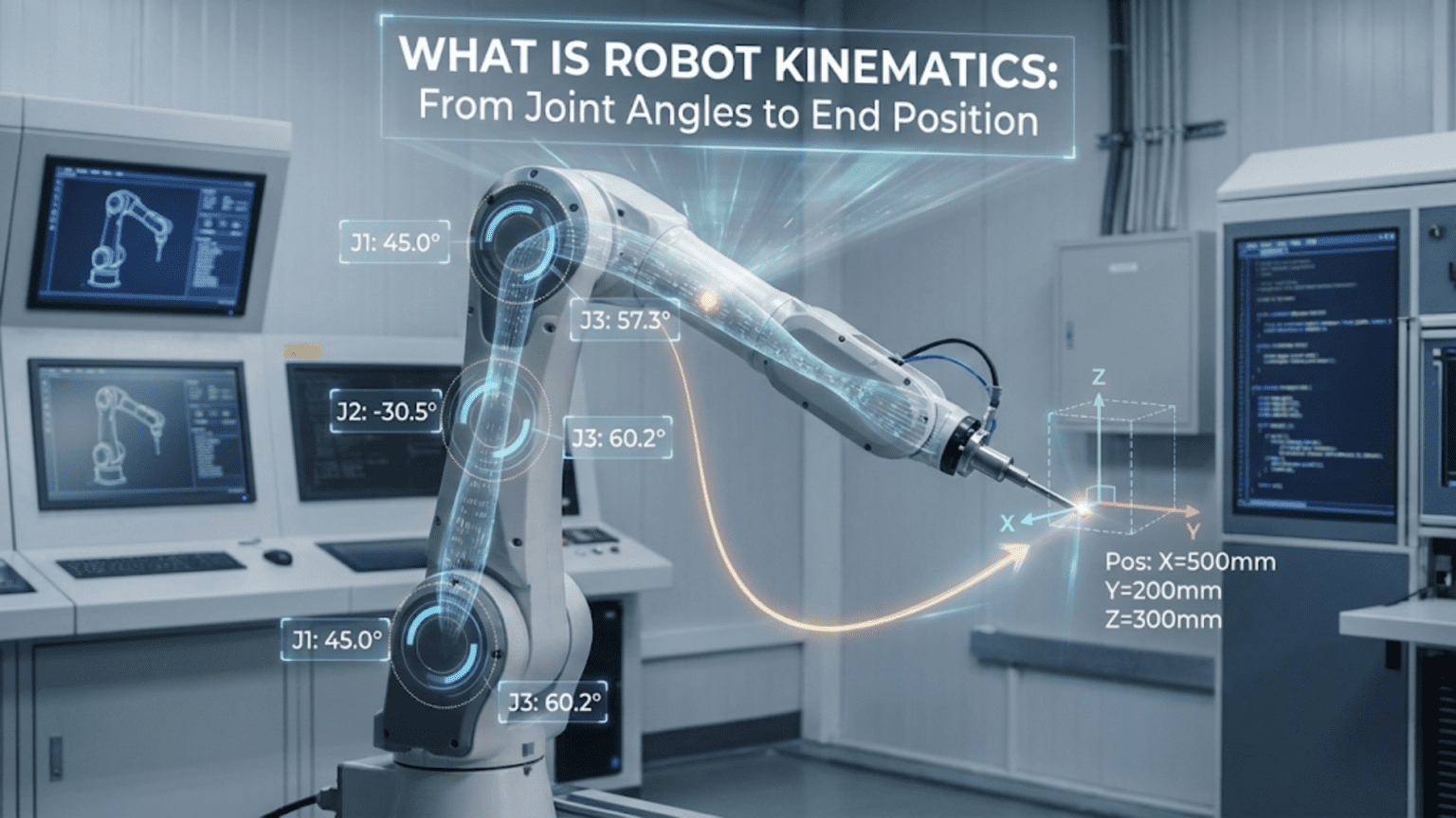
Robot kinematics is the mathematical study of motion in robotic systems—specifically the geometric relationships between joint angles and the resulting position and orientation of the robot’s end effector (tool or hand)—divided into forward kinematics (calculating where the end effector ends up given known joint angles) and inverse kinematics (calculating what joint angles are needed to place the end effector at a desired position). Mastering kinematics transforms robot programming from trial-and-error angle guessing into principled mathematical control where you command positions in real-world coordinates and the robot calculates the joint angles needed to get there.
You’ve built a two-joint robot arm and you want the gripper to move to a specific point in space—say, 20 centimeters to the right and 15 centimeters above the base. You could guess at joint angles, run the arm, measure where it ended up, adjust the angles, try again, and repeat. After dozens of iterations you might get close. For a simple arm, this trial-and-error approach is tedious but possible. For a six-joint industrial robot arm with hundreds of possible configurations for any given end-effector position, it becomes completely impractical. And if you need the end effector to follow a smooth path through space—tracing a straight line, following a curve, maintaining a precise orientation—guessing joint angles is simply impossible.
Robot kinematics solves this problem with mathematics. Rather than guessing, you describe the arm’s geometry precisely—link lengths, joint types, joint positions—and derive equations that convert between joint angle space (what the motors control) and Cartesian space (the physical world of X, Y, Z coordinates). These equations work in both directions: forward kinematics converts joint angles to end-effector position, and inverse kinematics converts desired end-effector position back to joint angles.
This article introduces robot kinematics from the ground up, using intuitive geometric reasoning before introducing trigonometry. We focus on planar (2D) and simple 3D robot arms that beginning and intermediate roboticists actually build, building toward the complete forward and inverse kinematics solutions you need to implement real position-controlled robot arms. By the end, you’ll understand why kinematics matters, how to derive it for simple arm configurations, how to implement it in Arduino code, how to plan straight-line and curved paths in task space, and how to extend your understanding toward more complex multi-joint systems.
The Language of Kinematics: Joints, Links, and Frames
Before deriving any equations, establishing precise terminology prevents confusion and makes the mathematics clearer.
Joints: The Degrees of Freedom
A joint is a connection between two rigid links that allows relative motion. In robotics, two joint types dominate:
Revolute joints (R): Allow rotation around a single axis. A hinge is a revolute joint. Servo motors and DC motors create revolute joints. The joint’s configuration is described by its angle θ (theta), measured from some reference direction. Most robot arms use exclusively revolute joints.
Prismatic joints (P): Allow linear sliding along a single axis. A piston or drawer slide is a prismatic joint. The joint’s configuration is described by its extension distance d. CNC machine axes use prismatic joints; robot arms occasionally include them for reach extension.
Degree of Freedom (DOF): Each independent joint contributes one degree of freedom. A 2-DOF arm has two joints, each independently controllable. To position an end effector at any point in 2D space and control its orientation, you need 3 DOF minimum. For full 3D positioning and orientation control, 6 DOF are required—which is why industrial robot arms typically have exactly six joints.
Links: The Rigid Segments
Links are the rigid structural elements connecting joints. Each link has:
Length (L): The distance between the joint centers at each end. Link length is fixed—it’s a physical property of your robot.
Index: Links are numbered from the base outward. Link 1 connects Joint 1 to Joint 2, Link 2 connects Joint 2 to Joint 3, and so on.
Reference Frames: Where We Measure From
A reference frame is a coordinate system—an origin point and three axes (X, Y, Z) that define directions for measurement.
World frame (base frame): Fixed to the robot’s base, this is the coordinate system in which we ultimately want to know the end-effector position. When you say “move to position X=20cm, Y=15cm,” you’re specifying coordinates in the world frame.
Joint frames: Each joint has a local coordinate system. Understanding how joint frames relate to each other is the core of formal kinematics. The Denavit-Hartenberg convention, used in advanced robotics, formalizes this systematically—it’s beyond our scope here but worth knowing exists as the next step.
End-effector frame: The coordinate system attached to the tool or gripper. The position and orientation of this frame relative to the world frame is what kinematics calculates.
Configuration Space vs. Task Space
These two complementary ways of describing robot state are fundamental to understanding kinematics:
Configuration space (joint space): Described by joint angles (θ₁, θ₂, θ₃, …). This is what motors directly control. A robot arm configuration is fully described by the set of all joint angles.
Task space (Cartesian space): Described by end-effector position (X, Y, Z) and orientation (roll, pitch, yaw). This is the space in which you specify where you want the robot to go.
Kinematics provides the mathematical bridge between these two spaces—converting in both directions. Forward kinematics maps from configuration space to task space. Inverse kinematics maps from task space back to configuration space.
Forward Kinematics: From Angles to Position
Forward kinematics answers: “Given these joint angles, where is the end effector?”
1-DOF System: The Simplest Case
A single revolute joint with a link of length L₁:
           End effector
           *
          /
         / L₁
        /
       / θ₁
  [J1]--------→ X axis
  |
| BaseThe end-effector position is simply:
- X = L₁ × cos(θ₁)
- Y = L₁ × sin(θ₁)
At θ₁ = 0°: end effector is at (L₁, 0) — pointing right along the X axis. At θ₁ = 90°: end effector is at (0, L₁) — pointing straight up. At θ₁ = 45°: end effector is at (L₁×0.707, L₁×0.707) — along the diagonal.
This single-joint case is trivial but establishes the pattern that extends to any number of joints: multiply each link length by the cosine/sine of its cumulative angle from the base reference.
2-DOF Planar Arm: The Foundation Case
A two-joint planar robot arm (both joints rotating in the same plane) is the most educational kinematics example and directly applies to many real hobby robot arms viewed from the side:
                    * End effector (x, y)
                   /
                  / L₂
                 /
            [J2]
           /
          / L₁
         /
    [J1]——→ X axis
    |
| BaseJoint 1 angle θ₁: Measured from the positive X axis to Link 1. Joint 2 angle θ₂: Measured from the direction of Link 1 to Link 2 (relative angle).
Finding the position of Joint 2 (end of Link 1):
- J2_x = L₁ × cos(θ₁)
- J2_y = L₁ × sin(θ₁)
Finding the end-effector position (end of Link 2): Link 2 makes an angle of (θ₁ + θ₂) with the X axis—because θ₂ is measured relative to Link 1’s direction, and Link 1 is already at angle θ₁ from the X axis. The angle of Link 2 from X is therefore their sum.
- X = L₁ × cos(θ₁) + L₂ × cos(θ₁ + θ₂)
- Y = L₁ × sin(θ₁) + L₂ × sin(θ₁ + θ₂)
These two equations are the complete forward kinematics for a 2-DOF planar arm. Given any θ₁ and θ₂, you can calculate exactly where the end effector is. No iteration, no approximation—exact geometry.
Numerical example: L₁ = 15cm, L₂ = 10cm, θ₁ = 45°, θ₂ = −30°
X = 15 × cos(45°) + 10 × cos(45° + (−30°)) = 15 × 0.7071 + 10 × cos(15°) = 10.61 + 10 × 0.9659 = 10.61 + 9.66 = 20.27 cm
Y = 15 × sin(45°) + 10 × sin(15°) = 15 × 0.7071 + 10 × 0.2588 = 10.61 + 2.59 = 13.20 cm
The end effector is at approximately (20.27 cm, 13.20 cm).
Forward Kinematics in Arduino Code
#include <math.h>

// Robot arm physical parameters (measure joint center to joint center)
const float L1 = 15.0;  // Link 1 length in cm
const float L2 = 10.0;  // Link 2 length in cm

struct Position2D {
  float x;
  float y;
};

// Forward kinematics: compute end effector position from joint angles (degrees)
Position2D forwardKinematics(float t1_deg, float t2_deg) {
  float t1 = t1_deg * PI / 180.0;  // Convert to radians
  float t2 = t2_deg * PI / 180.0;

  Position2D pos;
  pos.x = L1 * cos(t1) + L2 * cos(t1 + t2);
  pos.y = L1 * sin(t1) + L2 * sin(t1 + t2);
  return pos;
}

void setup() {
  Serial.begin(9600);
  Serial.println("2-DOF Forward Kinematics Calculator");
  Serial.println("====================================");

  // Test various configurations
  float testAngles[][2] = {
    {0,   0},    // Fully extended right
    {90,  0},    // Pointing straight up
    {45, -45},   // Diagonal, elbow bent inward
    {90, -90},   // Shoulder up, elbow folded — arm above base
    {0,   90},   // L-shape configuration
    {60,  30}    // Typical working configuration
  };

  for (int i = 0; i < 6; i++) {
    float t1 = testAngles[i][0];
    float t2 = testAngles[i][1];
    Position2D pos = forwardKinematics(t1, t2);

    Serial.print("θ1="); Serial.print(t1, 1);
    Serial.print("°, θ2="); Serial.print(t2, 1);
    Serial.print("° → X="); Serial.print(pos.x, 2);
    Serial.print("cm, Y="); Serial.print(pos.y, 2);
    Serial.println("cm");
  }
}

void loop() {}Sample output:
θ1=0.0°, θ2=0.0°   → X=25.00cm, Y=0.00cm
θ1=90.0°, θ2=0.0°  → X=0.00cm,  Y=25.00cm
θ1=45.0°, θ2=-45.0°→ X=20.27cm, Y=6.02cm
θ1=90.0°, θ2=-90.0°→ X=10.00cm, Y=15.00cm
θ1=0.0°, θ2=90.0°  → X=15.00cm, Y=10.00cm
θ1=60.0°, θ2=30.0° → X=9.82cm,  Y=21.83cm
Extending to 3-DOF Planar Arm
Adding a third joint and link follows the same additive pattern:
X = L₁×cos(θ₁) + L₂×cos(θ₁+θ₂) + L₃×cos(θ₁+θ₂+θ₃)
Y = L₁×sin(θ₁) + L₂×sin(θ₁+θ₂) + L₃×sin(θ₁+θ₂+θ₃)The third joint adds the ability to control end-effector orientation independently of position. With 3 DOF in a plane, you can reach any reachable point at any angle you choose—the third joint decouples position and orientation control.
3D Robot Arms: Adding Base Rotation
Most real robot arms operate in 3D. A common and powerful configuration adds a base rotation joint (rotating about the vertical Z axis) to a 2-DOF planar arm, giving 3 total DOF in 3D space:
Configuration: Base rotation (θ_base) + Shoulder (θ_shoulder) + Elbow (θ_elbow)Forward kinematics for this 3-DOF configuration:
First, calculate the arm’s reach in its own vertical plane using the 2D formula:
reach  = L₁×cos(θ_shoulder) + L₂×cos(θ_shoulder + θ_elbow)  (horizontal in arm plane)
height = L₁×sin(θ_shoulder) + L₂×sin(θ_shoulder + θ_elbow) (vertical, same in all planes)Then project the horizontal reach onto the X-Y ground plane using the base rotation:
X = reach × cos(θ_base)
Y = reach × sin(θ_base)
Z = height + base_heightstruct Position3D {
float x, y, z;
};
const float BASE_HEIGHT = 5.0; // cm, height of shoulder joint above ground
Position3D forwardKinematics3D(float base_deg, float shoulder_deg, float elbow_deg) {
float base = base_deg * PI / 180.0;
float shoulder = shoulder_deg * PI / 180.0;
float elbow = elbow_deg * PI / 180.0;
float reach = L1 * cos(shoulder) + L2 * cos(shoulder + elbow);
float height = L1 * sin(shoulder) + L2 * sin(shoulder + elbow);
Position3D pos;
pos.x = reach * cos(base);
pos.y = reach * sin(base);
pos.z = BASE_HEIGHT + height;
return pos;
}Inverse Kinematics: From Position to Angles
Inverse kinematics answers the harder question: “Given a desired end-effector position, what joint angles should I command?”
This direction is harder than forward kinematics for three reasons. First, multiple solutions typically exist—most positions can be reached in more than one configuration (the classic elbow-up versus elbow-down choice). Second, singularities occur where solutions are degenerate or infinite. Third, some positions are simply unreachable—the math produces imaginary numbers as an unambiguous signal.
Despite these challenges, closed-form geometric inverse kinematics for 2-DOF and simple 3-DOF arms is completely tractable using trigonometry and the law of cosines.
Geometric Inverse Kinematics for 2-DOF Arm
Given desired position (x, y) and known link lengths L₁ and L₂, find θ₁ and θ₂.
Step 1: Find θ₂ using the law of cosines
The distance from the base to the end effector is:
D = √(x² + y²)The three points—the base joint, the elbow joint, and the end effector—form a triangle with sides L₁, L₂, and D. Applying the law of cosines:
D² = L₁² + L₂² − 2×L₁×L₂×cos(180° − θ₂)
D² = L₁² + L₂² + 2×L₁×L₂×cos(θ₂)

Solving for θ₂:
cos(θ₂) = (D² − L₁² − L₂²) / (2×L₁×L₂)
θ₂ = ±arccos((D² − L₁² − L₂²) / (2×L₁×L₂))The ± gives exactly two solutions: elbow-up (positive θ₂, elbow above the line from base to end effector) and elbow-down (negative θ₂, elbow below that line). Both are geometrically valid; you choose based on your physical constraints.
Step 2: Find θ₁ using atan2
With θ₂ known:
α = atan2(y, x)                                        — direction to target
β = atan2(L₂×sin(θ₂), L₁ + L₂×cos(θ₂))              — elbow correction angle

For elbow-up:   θ₁ = α − β
For elbow-down: θ₁ = α + βWhy atan2 instead of arctan: The atan2(y, x) function correctly handles all four quadrants, returning angles from −π to +π. Regular arctan only spans −π/2 to +π/2 and loses quadrant information, producing wrong answers for targets in the left half of the workspace. Always use atan2 in kinematics code.
Complete Inverse Kinematics Implementation
#include <math.h>
#include <Servo.h>

const float L1 = 15.0;  // cm
const float L2 = 10.0;  // cm

Servo shoulder;
Servo elbow;

struct IKResult {
  bool  reachable;
  float theta1;    // degrees
  float theta2;    // degrees
  bool  elbowUp;
};

// Compute inverse kinematics for a 2-DOF planar arm
IKResult inverseKinematics(float x, float y, bool preferElbowUp = true) {
  IKResult result;
  result.reachable = false;

  float D       = sqrt(x * x + y * y);
  float maxReach = L1 + L2;
  float minReach = fabs(L1 - L2);

  if (D > maxReach) {
    Serial.print("Too far: D="); Serial.print(D);
    Serial.print(" max="); Serial.println(maxReach);
    return result;
  }
  if (D < minReach) {
    Serial.print("Too close: D="); Serial.print(D);
    Serial.print(" min="); Serial.println(minReach);
    return result;
  }

  // Law of cosines → θ₂
  float cosTheta2 = (D*D - L1*L1 - L2*L2) / (2.0 * L1 * L2);
  cosTheta2 = constrain(cosTheta2, -1.0, 1.0);  // Guard against floating-point drift

  float theta2_rad = preferElbowUp ? acos(cosTheta2) : -acos(cosTheta2);

  // Geometry → θ₁
  float alpha = atan2(y, x);
  float beta  = atan2(L2 * sin(theta2_rad), L1 + L2 * cos(theta2_rad));
  float theta1_rad = alpha - beta;

  result.theta1   = theta1_rad * 180.0 / PI;
  result.theta2   = theta2_rad * 180.0 / PI;
  result.reachable = true;
  result.elbowUp  = preferElbowUp;
  return result;
}

// Joint limits (physical servo constraints)
const float THETA1_MIN = 0,   THETA1_MAX = 180;
const float THETA2_MIN = -120, THETA2_MAX = 120;

bool withinLimits(float t1, float t2) {
  return (t1 >= THETA1_MIN && t1 <= THETA1_MAX &&
          t2 >= THETA2_MIN && t2 <= THETA2_MAX);
}

// Move arm to (x, y); try elbow-up first, fall back to elbow-down
bool moveToPosition(float x, float y) {
  IKResult ik = inverseKinematics(x, y, true);

  if (!ik.reachable || !withinLimits(ik.theta1, ik.theta2)) {
    ik = inverseKinematics(x, y, false);  // Try elbow-down
  }
  if (!ik.reachable || !withinLimits(ik.theta1, ik.theta2)) {
    Serial.println("Position unreachable within joint limits");
    return false;
  }

  shoulder.write((int)ik.theta1);
  elbow.write((int)(90 + ik.theta2));  // Offset: servo center = 90°

  Serial.print("→ ("); Serial.print(x,1); Serial.print(", ");
  Serial.print(y,1); Serial.print(")  θ1="); Serial.print(ik.theta1,1);
  Serial.print("° θ2="); Serial.print(ik.theta2,1); Serial.println("°");
  return true;
}

void setup() {
  shoulder.attach(9);
  elbow.attach(10);
  Serial.begin(9600);
  Serial.println("2-DOF IK Arm Ready");
  moveToPosition(L1 + L2, 0);  // Home: fully extended
  delay(1000);
}

void loop() {
  float targets[][2] = {{20,10},{15,15},{10,20},{18,5},{22,8}};
  for (int i = 0; i < 5; i++) {
    moveToPosition(targets[i][0], targets[i][1]);
    delay(1500);
  }
}Inverse Kinematics for the 3-DOF Arm
Extending IK to the 3-DOF arm (base + 2D planar) is elegant because it decomposes into independent sub-problems:
struct IKResult3D {
  bool  reachable;
  float base;      // degrees
  float shoulder;  // degrees
  float elbow;     // degrees
};

IKResult3D inverseKinematics3D(float x, float y, float z) {
  IKResult3D result;
  result.reachable = false;

  // Step 1: Base angle from horizontal ground projection
  result.base = atan2(y, x) * 180.0 / PI;

  // Step 2: Horizontal reach and vertical height in the arm's plane
  float reach  = sqrt(x*x + y*y);
  float height = z - BASE_HEIGHT;

  // Step 3: Standard 2D IK on (reach, height)
  IKResult ik2D = inverseKinematics(reach, height, true);
  if (!ik2D.reachable) return result;

  result.shoulder  = ik2D.theta1;
  result.elbow     = ik2D.theta2;
  result.reachable = true;
  return result;
}Workspace Analysis: Knowing What Your Arm Can Reach
The workspace is the complete set of positions the end effector can physically reach. Understanding it prevents commanding impossible positions and informs design decisions—arm lengths, joint limit choices, and mounting position all shape the workspace.
Reachability Bounds
For a 2-DOF arm, the reachable workspace is an annular region (ring) in the plane:
Minimum reach: D_min = |L₁ − L₂|   (arm fully folded back on itself)
Maximum reach: D_max = L₁ + L₂ (arm fully extended)With L₁ = 15cm and L₂ = 10cm:
- D_max = 25 cm
- D_min = 5 cm
Every point in the ring from 5cm to 25cm from the base joint (in the reachable angular sector) can be reached. Points outside this ring cannot.
Singularities: The Problematic Boundaries
Singularities are configurations where the robot loses a degree of freedom or where velocity amplification becomes infinite.
Fully extended singularity (D = L₁ + L₂): The arm is completely straight. Joint 2 is at 0° and cannot contribute to motion perpendicular to the arm. Very small end-effector movements perpendicular to the arm require very large Joint 1 rotations—velocity amplification approaches infinity.
Fully folded singularity (D = |L₁ − L₂|): The arm doubles back completely. Similarly ill-conditioned.
Practical consequence: Paths that pass near singularities produce sudden, large joint velocity requirements—jerky motion that can stress mechanisms and lose steps. Keep operating positions comfortably within the workspace interior.
bool nearSingularity(float x, float y, float margin = 2.0) {
  float D = sqrt(x*x + y*y);
  return (D > L1 + L2 - margin) || (D < fabs(L1 - L2) + margin);
}Workspace Visualization on Serial Monitor
void printWorkspaceMap() {
  float maxR = L1 + L2;
  float minR = fabs(L1 - L2);
  float scale = 2.0;  // cm per character

  Serial.println("Workspace (O=reachable, .=unreachable)");
  for (int row = (int)(maxR/scale); row >= -(int)(maxR/scale*0.3); row--) {
    for (int col = -(int)(maxR/scale*0.3); col <= (int)(maxR/scale); col++) {
      float x = col * scale;
      float y = row * scale;
      float D = sqrt(x*x + y*y);
      Serial.print((D <= maxR && D >= minR) ? "O" : ".");
    }
    Serial.println();
  }
}Straight-Line Path Planning in Task Space
The real power of kinematics emerges when you command the end effector to follow a specific geometric path—something impossible with pure joint-space control.
Linear Interpolation
Move the end effector in a straight line between two points by computing IK for a dense sequence of interpolated positions:
void moveLinear(float x0, float y0, float x1, float y1,
                int numSteps, int stepDelay_ms) {
  Serial.print("Linear: ("); Serial.print(x0,1);
  Serial.print(","); Serial.print(y0,1);
  Serial.print(") → ("); Serial.print(x1,1);
  Serial.print(","); Serial.print(y1,1); Serial.println(")");

  for (int i = 0; i <= numSteps; i++) {
    float t = (float)i / numSteps;
    float x = x0 + t * (x1 - x0);
    float y = y0 + t * (y1 - y0);

    if (nearSingularity(x, y)) {
      Serial.println("WARNING: near singularity");
    }

    if (!moveToPosition(x, y)) {
      Serial.println("Path aborted — unreachable point");
      return;
    }
    delay(stepDelay_ms);
  }
  Serial.println("Linear move complete");
}Circular Arc Path
Trace a circular arc by sweeping an angle parameter:
void moveArc(float cx, float cy, float radius,
             float startAngle_deg, float endAngle_deg,
             int numSteps, int stepDelay_ms) {
  for (int i = 0; i <= numSteps; i++) {
    float t     = (float)i / numSteps;
    float angle = (startAngle_deg + t * (endAngle_deg - startAngle_deg)) * PI / 180.0;
    float x     = cx + radius * cos(angle);
    float y     = cy + radius * sin(angle);
    moveToPosition(x, y);
    delay(stepDelay_ms);
  }
}

// Example: full circle of radius 5 cm centered at (15, 8)
// moveArc(15, 8, 5, 0, 360, 72, 60);Smooth Joint-Space Interpolation
When commanded positions are close together but change quickly, smooth joint interpolation prevents vibration:
void smoothMoveJoints(float targetT1, float targetT2,
                      int steps, int stepDelay_ms) {
  float startT1 = (float)shoulder.read();
  float startT2 = (float)elbow.read() - 90.0;  // Remove servo offset

  for (int i = 1; i <= steps; i++) {
    float t  = (float)i / steps;
    float t1 = startT1 + t * (targetT1 - startT1);
    float t2 = startT2 + t * (targetT2 - startT2);
    shoulder.write((int)t1);
    elbow.write((int)(t2 + 90));
    delay(stepDelay_ms);
  }
}Calibration and Practical Implementation
Kinematic equations are only as accurate as the measurements and calibration feeding them.
Measure Link Lengths Precisely
Measure L₁ and L₂ as the distance between joint rotation axis centers—not the physical length of the structural member. A 1mm error in a link length propagates directly as end-effector position error at every configuration.
Calibrate Servo Zero Offsets
Real servos don’t perfectly align their mechanical output with their commanded angle. Calibrate each servo:
// Offsets in degrees (positive = servo reads too high)
const int SHOULDER_OFFSET =  3;
const int ELBOW_OFFSET    = -2;

void writeJoint(Servo& srv, float angle_deg, int offset) {
  int cmd = constrain((int)angle_deg + offset, 0, 180);
  srv.write(cmd);
}Validate IK with Forward Kinematics
Always cross-check computed IK angles by running forward kinematics on them and verifying the result matches your target:
bool verifyIK(float targetX, float targetY,
              float theta1, float theta2, float tol = 0.5) {
  Position2D actual = forwardKinematics(theta1, theta2);
  if (fabs(actual.x - targetX) > tol || fabs(actual.y - targetY) > tol) {
    Serial.print("IK verify FAIL: got (");
    Serial.print(actual.x,2); Serial.print(",");
    Serial.print(actual.y,2); Serial.println(")");
    return false;
  }
  return true;
}Comparison Table: Kinematics Approaches
| Approach | Complexity | Accuracy | Compute Cost | Best For |
|---|---|---|---|---|
| Trial-and-error tuning | None | Low | None | Static poses only |
| Forward kinematics | Low | Exact (given angles) | Very Low | Position display, simulation |
| Geometric IK — 2-DOF | Medium | High | Very Low | 2-joint planar arms |
| Geometric IK — 3-DOF | Medium-High | High | Low | Arms with base rotation |
| Numerical IK (Jacobian) | High | Medium-High | Medium | 4–6 DOF general arms |
| Pre-computed IK table | Low (after setup) | Medium | Minimal | Repeated known positions |
| DH Parameter method | Very High | Exact | Low-Medium | Formal multi-joint derivation |
Conclusion: Kinematics as the Mathematical Foundation of Robot Arms
Robot kinematics provides the mathematical bridge between the physical space where work happens and the joint space that motors control. Without it, positioning a robot arm is trial and error; with it, you command positions in intuitive Cartesian coordinates and let well-understood mathematics determine the required joint angles precisely and instantly.
Forward kinematics builds on a simple additive chain: each link contributes its length projected onto X and Y by the cosine and sine of its cumulative angle from the base. The equations for two-joint, three-joint, and more complex arms all follow the same structure. Inverse kinematics reverses the process through the law of cosines and atan2, revealing workspace boundaries, dual solutions, and singularities as natural mathematical consequences rather than mysterious behaviors.
The 2-DOF planar arm kinematics presented here is genuinely useful for real robots—many hobby and educational arms are exactly this configuration and the equations work directly. The extension to 3-DOF with base rotation handles the vast majority of desktop robot arms and provides the geometric intuition needed to approach more complex systems confidently.
Path planning demonstrates the transformative power of kinematics. Once you can compute joint angles for any single reachable point, you can compute them for a dense sequence of points along any geometric path—straight lines, arcs, spirals—creating smooth, predictable end-effector motion that would be completely impossible through direct joint-angle commands.
More complex systems with 4, 5, or 6 degrees of freedom require Denavit-Hartenberg parameters for systematic frame assignment and Jacobian-based methods for velocity kinematics and general IK. But the conceptual foundation transfers directly: workspace, singularities, multiple solution branches, and the forward/inverse duality all appear in the same forms. Master kinematics for 2-DOF and 3-DOF arms and you have the geometric intuition that makes advanced robotic manipulation understandable rather than mysterious—the gateway to designing and controlling any robot arm you can imagine.