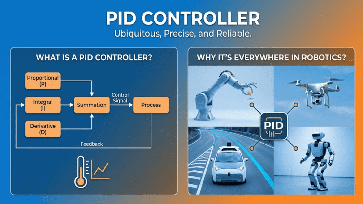
A PID controller is a feedback control algorithm that calculates a corrective output using three mathematical terms: the Proportional term (responding to current error), the Integral term (responding to accumulated past error), and the Derivative term (responding to the rate of error change), combining them to eliminate the difference between a desired setpoint and a measured process value. PID controllers are the most widely deployed control algorithm in all of engineering, appearing in robot motor drives, drone stabilization, industrial automation, temperature regulation, and virtually every system that requires precise, automatic control.
Introduction
You’re watching a professional drone pilot hover a quadrotor at a fixed point in the air. The drone sits perfectly still despite wind gusts, small disturbances, and the inherent instability of its four-rotor design. What you’re seeing is a PID controller—actually several of them running simultaneously—making hundreds of tiny corrections every second to keep the drone exactly where it should be.
You’re watching a CNC machine carve a complex shape from aluminum, the cutting tool following a programmed path with sub-millimeter precision at high speed. PID controllers on each axis continuously compare actual position to commanded position and drive the motors to minimize the difference.
You’re watching a robot arm weld two pieces of steel together, the torch following a precise seam as the arm moves smoothly despite varying loads and friction at each joint. PID controllers at every joint keep each axis precisely on its programmed trajectory.
The PID controller is the workhorse of modern control engineering. Invented in the early twentieth century for ship steering control, refined over decades of industrial application, and now running in billions of embedded systems worldwide, it solves one of the most fundamental challenges in all of technology: how do you get a physical system to do exactly what you want, reliably, even when the world doesn’t cooperate?
Understanding PID control is one of the highest-leverage skills in robotics. Once you truly understand it—not just the equation but the intuition behind each term—you can tune motor controllers, stabilize drones, build line-following robots, implement temperature control, and approach virtually any continuous control problem with confidence. This article builds that understanding from the ground up.
The Problem PID Control Solves
Before diving into the algorithm itself, it’s worth being precise about the problem that PID control addresses.
You have a system with a process variable—some measurable quantity you want to control. This might be motor speed, joint angle, robot heading, temperature, altitude, or any other continuously varying physical quantity.
You have a setpoint—the value you want the process variable to reach and maintain.
You have an actuator—something you can command to influence the process variable. This might be motor voltage, a heater power level, a control surface deflection, or any other controllable input to the system.
The control challenge: given a measurement of the current process variable and knowledge of the desired setpoint, what command should you send to the actuator at each moment to drive the process variable to the setpoint and keep it there, as accurately and smoothly as possible, in the presence of disturbances, noise, and model uncertainty?
A simple approach—”apply maximum actuator command when below setpoint, zero when above”—produces the bang-bang controller discussed in the previous article. It works but causes perpetual oscillation. A proportional controller—”apply command proportional to the current error”—is smoother but leaves a persistent residual error. PID control adds two more terms that eliminate these remaining shortcomings, producing a controller that is stable, accurate, and responsive.
The Three Terms of PID Control
The PID algorithm combines three separate calculations, each responding to a different aspect of the error signal.
The Error Signal
Everything starts with the error—the difference between the desired setpoint and the current measured value:
Error(t) = Setpoint - Measurement(t)The error is positive when the process variable is below the setpoint (more output needed) and negative when it’s above the setpoint (less output needed). It changes continuously as the system evolves.
The Proportional Term (P)
The proportional term produces an output directly proportional to the current error:
P_output = Kp × Error(t)The parameter Kp is the proportional gain. It scales how aggressively the controller responds to current error. A high Kp produces strong, fast corrections for any given error. A low Kp produces mild, gentle corrections.
Intuition: The proportional term asks, “How far off am I right now?” It’s like a spring—the further you pull it from equilibrium, the harder it pulls back. Large error produces large correction. Small error produces small correction.
The fundamental limitation: Proportional control alone almost always leaves a steady-state error. Consider a motor speed controller: to maintain a target speed against friction, the controller must continuously output some non-zero drive signal. But if error approaches zero, the P term also approaches zero, and with zero output the motor stops. The system settles at some error value where the P output just barely overcomes friction—never quite reaching the setpoint. This residual error is called offset or steady-state error, and it’s the P term’s inherent limitation.
float proportionalTerm(float setpoint, float measurement, float Kp) {
  float error = setpoint - measurement;
  return Kp * error;
}The Integral Term (I)
The integral term accumulates error over time and produces an output proportional to the total accumulated error:
I_output = Ki × ∫Error(t)dtIn discrete-time code (which is how microcontrollers implement this), the integral becomes a running sum:
integral += Error × deltaTime
I_output = Ki × integralThe parameter Ki scales the strength of the integral response. A high Ki makes the integral term respond quickly to accumulated error. A low Ki makes it respond slowly.
Intuition: The integral term asks, “Have I been off target for a long time?” It measures persistent error that the proportional term hasn’t eliminated. Think of it as memory—it remembers every past error and adds them up. If the system has been sitting 2 RPM below target for 5 seconds, the integral has accumulated a significant value, even though the current error might seem modest. This accumulated value pushes the output higher until the error is truly eliminated and the integral stops growing.
What the integral term fixes: Steady-state error. By accumulating error over time, the integral term keeps increasing the controller output until the process variable actually reaches the setpoint. Once it reaches the setpoint and error goes to zero, the integral stops accumulating—it maintains whatever value it reached, and that value is precisely what’s needed to overcome the constant opposing forces (friction, gravity, etc.) that were causing the steady-state error.
The integral term’s complication: Windup. If the system is far from the setpoint for a long time—for example, during startup when a motor is at zero speed and needs to reach 100 RPM—the integral accumulates a very large value. When the system finally approaches the setpoint, this large accumulated integral continues driving strong output even after the error has gone to zero, causing significant overshoot. This problem is called integral windup, and managing it (through integral clamping or anti-windup techniques) is one of the key practical challenges of PID implementation.
float integralSum = 0;
float lastTime = 0;

float integralTerm(float error, float Ki, float maxIntegral) {
  float currentTime = millis() / 1000.0;
  float deltaTime = currentTime - lastTime;
  lastTime = currentTime;

  integralSum += error * deltaTime;

  // Anti-windup: clamp the integral sum
  integralSum = constrain(integralSum, -maxIntegral, maxIntegral);

  return Ki * integralSum;
}The Derivative Term (D)
The derivative term responds to the rate of change of the error—how quickly the error is currently changing:
D_output = Kd × d(Error)/dtIn discrete-time implementation:
D_output = Kd × (Error - previousError) / deltaTimeThe parameter Kd scales the derivative response. A high Kd produces strong damping for rapid error changes. A low Kd produces mild damping.
Intuition: The derivative term asks, “How fast is the error changing right now?” It predicts where the error is heading. If the error is currently large but shrinking rapidly, the derivative term knows the system is on its way to the setpoint and reduces the output preemptively—preventing overshoot. If the error is currently small but growing fast (perhaps a sudden disturbance), the derivative term responds aggressively even before the error becomes large.
Think of it as a braking force. Without the derivative term, a proportional controller drives hard toward the setpoint but doesn’t know when to ease off, causing overshoot and oscillation. The derivative term senses the approaching momentum and applies brakes, producing a smooth, overdamped approach.
The derivative term’s complication: Noise sensitivity. The derivative calculates the rate of change between consecutive measurements. If sensor noise causes small, rapid fluctuations in the measurement, the derivative amplifies these fluctuations into large, rapid changes in the controller output. This can cause the actuator to chatter noisily and inefficiently. The solution is to filter the derivative calculation—often by applying a low-pass filter to the derivative term or to the sensor reading before differentiation.
A commonly used approach is derivative-on-measurement rather than derivative-on-error: calculating the derivative of the measurement signal rather than the error signal. This avoids derivative kicks when the setpoint changes suddenly (which would create a step change in error and a huge derivative spike):
float lastMeasurement = 0;

float derivativeTerm(float measurement, float Kd, float deltaTime) {
  // Derivative-on-measurement avoids setpoint kick
  float dMeasurement = (measurement - lastMeasurement) / deltaTime;
  lastMeasurement = measurement;

  return -Kd * dMeasurement;  // Negative because we want to oppose measurement increase
}The Complete PID Equation
Combining all three terms gives the complete PID controller output:
Output = Kp×Error + Ki×∫Error dt + Kd×d(Error)/dtOr in words: the controller output equals the proportional gain times current error, plus the integral gain times accumulated past error, plus the derivative gain times the rate of error change.
Each term contributes differently:
- P provides immediate response to current error — the engine
- I eliminates persistent steady-state error — the corrector
- D dampens oscillation and prevents overshoot — the brake
Together, they form a complete, self-correcting control law that can be applied to an enormous range of physical systems.
Complete PID Implementation in Arduino
Here is a full, practical PID controller implementation suitable for real robotics projects:
// Complete PID Controller Implementation
// Suitable for motor speed, position, line following, etc.

class PIDController {
private:
  float Kp, Ki, Kd;
  float setpoint;
  float integralSum;
  float lastMeasurement;
  float lastTime;
  float outputMin, outputMax;
  float integralMin, integralMax;

public:
  PIDController(float kp, float ki, float kd, float outMin, float outMax) {
    Kp = kp;
    Ki = ki;
    Kd = kd;
    outputMin = outMin;
    outputMax = outMax;
    integralMin = outMin / ki;  // Scale integral limits by Ki
    integralMax = outMax / ki;
    integralSum = 0;
    lastMeasurement = 0;
    lastTime = 0;
    setpoint = 0;
  }

  void setSetpoint(float sp) {
    setpoint = sp;
  }

  void setGains(float kp, float ki, float kd) {
    // Reset integral when gains change to avoid windup
    if (Ki != ki) integralSum = 0;
    Kp = kp;
    Ki = ki;
    Kd = kd;
  }

  void reset() {
    integralSum = 0;
    lastMeasurement = 0;
    lastTime = millis() / 1000.0;
  }

  float compute(float measurement) {
    float currentTime = millis() / 1000.0;
    float deltaTime = currentTime - lastTime;

    // Prevent division by zero on first call
    if (deltaTime <= 0) deltaTime = 0.001;
    lastTime = currentTime;

    // Calculate error
    float error = setpoint - measurement;

    // Proportional term
    float pTerm = Kp * error;

    // Integral term with anti-windup clamping
    integralSum += error * deltaTime;
    integralSum = constrain(integralSum, integralMin, integralMax);
    float iTerm = Ki * integralSum;

    // Derivative term (on measurement to avoid setpoint kick)
    float dMeasurement = (measurement - lastMeasurement) / deltaTime;
    float dTerm = -Kd * dMeasurement;
    lastMeasurement = measurement;

    // Total output
    float output = pTerm + iTerm + dTerm;

    // Clamp output to valid range
    output = constrain(output, outputMin, outputMax);

    return output;
  }

  // Debugging: print current state
  void printState(float measurement) {
    float error = setpoint - measurement;
    Serial.print("SP:"); Serial.print(setpoint);
    Serial.print(" PV:"); Serial.print(measurement);
    Serial.print(" Err:"); Serial.print(error);
    Serial.print(" I:"); Serial.print(integralSum);
    Serial.print(" Out:"); Serial.println(Kp*error + Ki*integralSum);
  }
};

// -------- Example: Motor Speed PID Controller --------

const int MOTOR_PWM_PIN = 5;
const int MOTOR_DIR_PIN = 4;
const int ENCODER_PIN = 2;

volatile long encoderCount = 0;
long lastCount = 0;
unsigned long lastSpeedTime = 0;
float measuredRPM = 0;
const int ENCODER_CPR = 20;  // Counts per revolution

PIDController speedPID(2.0, 0.8, 0.05, 0, 255);

void encoderISR() { encoderCount++; }

void setup() {
  Serial.begin(9600);
  pinMode(MOTOR_PWM_PIN, OUTPUT);
  pinMode(MOTOR_DIR_PIN, OUTPUT);
  pinMode(ENCODER_PIN, INPUT_PULLUP);
  attachInterrupt(digitalPinToInterrupt(ENCODER_PIN), encoderISR, RISING);

  digitalWrite(MOTOR_DIR_PIN, HIGH);  // Forward

  speedPID.setSetpoint(120.0);  // Target: 120 RPM
  lastSpeedTime = millis();
}

void loop() {
  unsigned long now = millis();

  // Update speed measurement and PID every 50ms
  if (now - lastSpeedTime >= 50) {
    long countDelta = encoderCount - lastCount;
    lastCount = encoderCount;
    float dt = (now - lastSpeedTime) / 1000.0;
    lastSpeedTime = now;

    // RPM = (counts / CPR) / dt * 60
    measuredRPM = (countDelta / (float)ENCODER_CPR) / dt * 60.0;

    // Compute PID output
    float pwmOutput = speedPID.compute(measuredRPM);
    analogWrite(MOTOR_PWM_PIN, (int)pwmOutput);

    speedPID.printState(measuredRPM);
  }
}This implementation is clean, reusable, and ready for real projects. The PIDController class handles all the math, anti-windup clamping, and derivative-on-measurement automatically. You instantiate it with gains and output limits, call setSetpoint() with your target, and call compute() with each new measurement to get the corrective output.
Understanding PID Behavior: What Each Term Actually Does
To truly master PID, you need intuitive mental models for how each term affects system behavior. Let’s walk through a concrete scenario: bringing a motor from rest to a target speed of 100 RPM.
Phase 1: Startup (large error, error decreasing)
At time zero, the motor is stopped. Error = 100 RPM.
- P term: Large positive output (Kp × 100). Motor drives hard toward the target. Good.
- I term: Integral is zero at startup, begins accumulating. Small initial contribution.
- D term: The measurement (actual RPM) starts increasing rapidly. The derivative of a rapidly increasing measurement is a large negative value, which the D term uses to apply “brakes.” This prevents the motor from rushing past the target.
Phase 2: Approaching Target (error shrinking rapidly)
Motor is at 80 RPM, rapidly approaching 100 RPM.
- P term: Error is 20 RPM. Output is moderate (Kp × 20).
- I term: Has accumulated some error from the startup phase. Adds a positive contribution.
- D term: Measurement still increasing, applying braking. Reduces total output to prevent overshoot.
Phase 3: At or Near Target (small, stable error)
Motor is at 98 RPM and stable.
- P term: Error is 2 RPM. Small positive output.
- I term: Has accumulated enough to overcome motor friction. Provides the “steady push” that keeps the motor at speed even with zero setpoint velocity from the P term.
- D term: Measurement is stable (not changing). Derivative ≈ 0. No contribution.
Phase 4: Disturbance (sudden load added)
A load is suddenly applied to the motor shaft. Speed drops to 90 RPM.
- P term: Error suddenly jumps to 10 RPM. Increases output.
- I term: Begins accumulating additional error. Increases gradually.
- D term: Measurement dropped sharply—the derivative is large and negative, meaning the measurement is decreasing fast. The D term adds a strong positive contribution (opposing the rapid decrease), responding to the disturbance immediately even before the error has grown large.
This is the power of PID working as a team: the D term responds immediately to rapid changes, the P term handles the current magnitude, and the I term eliminates any persistent offset.
The Crucial Skill: PID Tuning
Having the right controller structure is half the battle. The other half is setting the right gain values—Kp, Ki, and Kd. This process is called tuning, and it’s one of the most important practical skills in robotics control.
The Manual Tuning Method (Ziegler-Nichols Inspired)
The most common manual tuning approach follows a structured sequence:
Step 1: Start with all gains at zero. Set Ki = 0, Kd = 0, Kp = 0. The motor (or other system) will be uncontrolled.
Step 2: Increase Kp until the system oscillates. Gradually increase Kp while watching the system’s response. At first, response will be sluggish. As Kp increases, response gets faster. Eventually the system will begin to oscillate—it’ll reach the setpoint, overshoot, correct, overshoot in the other direction, and repeat continuously. Note this Kp value as Ku (ultimate gain) and the oscillation period as Tu.
Step 3: Set Kp to half the ultimate gain. Set Kp = 0.6 × Ku. This gives a good proportional response without instability.
Step 4: Add derivative gain. Set Kd = Kp × Tu / 8. The D term dampens the oscillations you’d otherwise see with proportional control alone. Increase Kd until the system response becomes crisp without excessive oscillation.
Step 5: Add integral gain slowly. Set Ki = 2 × Kp / Tu. The I term eliminates steady-state error. Add it last because it can destabilize a system if too high. Increase slowly until steady-state error is eliminated without excessive overshoot.
Step 6: Fine-tune iteratively. Make small adjustments to each gain while observing system behavior. Use the behavioral signatures in the table below to diagnose and correct specific problems.
Behavioral Signatures for Diagnosis
| Symptom | Likely Cause | Fix |
|---|---|---|
| Slow, sluggish response | Kp too low | Increase Kp |
| Large, persistent overshoot | Kp too high or Kd too low | Decrease Kp or increase Kd |
| Continuous oscillation (never settles) | Kp too high | Decrease Kp |
| Steady-state error remains | Ki too low or zero | Increase Ki |
| Slow drift toward setpoint | Ki too low | Increase Ki |
| Overshoot after disturbance, then OK | Ki too high | Decrease Ki |
| Noisy, chattering actuator | Kd too high or sensor noise | Decrease Kd or filter sensor |
| Sluggish recovery from disturbance | Kd too low | Increase Kd |
| Integral windup (huge overshoot on startup) | No anti-windup | Add integral clamping |
| Setpoint step causes large derivative spike | Derivative on error | Switch to derivative-on-measurement |
Real Robotics Applications of PID Control
Application 1: Line-Following Robot
A line-following robot uses a sensor array to detect the position of a line beneath it. The position of the line relative to the robot’s center is the error signal. PID control keeps the robot centered on the line by adjusting the relative speeds of the left and right motors.
// Line follower PID implementation
// Sensor array: 5 sensors returning values 0-4095
// Position: weighted average gives a value from 0 (far left) to 4000 (far right)
// Target: 2000 (center)

const int NUM_SENSORS = 5;
const int SENSOR_PINS[] = {A0, A1, A2, A3, A4};
const int BASE_SPEED = 180;
const int MAX_SPEED = 255;
const int MIN_SPEED = 0;

float Kp = 0.08;
float Ki = 0.0002;
float Kd = 1.2;

float lastError = 0;
float integral = 0;

int readLinePosition() {
  int values[NUM_SENSORS];
  long weightedSum = 0;
  long sum = 0;

  for (int i = 0; i < NUM_SENSORS; i++) {
    values[i] = analogRead(SENSOR_PINS[i]);
    weightedSum += (long)values[i] * i * 1000;
    sum += values[i];
  }

  if (sum == 0) return 2000;  // No line detected, use last known center
  return weightedSum / sum;
}

void loop() {
  int position = readLinePosition();
  float error = 2000 - position;  // 0 = centered, + = line to left, - = line to right

  integral += error;
  integral = constrain(integral, -5000, 5000);  // Anti-windup

  float derivative = error - lastError;
  lastError = error;

  float correction = (Kp * error) + (Ki * integral) + (Kd * derivative);

  int leftSpeed  = constrain(BASE_SPEED + correction, MIN_SPEED, MAX_SPEED);
  int rightSpeed = constrain(BASE_SPEED - correction, MIN_SPEED, MAX_SPEED);

  setMotors(leftSpeed, rightSpeed);

  Serial.print("Pos:"); Serial.print(position);
  Serial.print(" Err:"); Serial.print(error);
  Serial.print(" Corr:"); Serial.println(correction);
}The beauty of this implementation: regardless of curve sharpness, surface color variation, or motor differences, the PID loop continuously calculates the correction needed and adjusts motor speeds to keep the line centered in the sensor array.
Application 2: Drone Altitude Hold
A drone hovering at a fixed altitude uses a barometer or ultrasonic sensor to measure current altitude. The PID controller compares measured altitude to the target altitude and adjusts throttle output to maintain the setpoint.
// Simplified altitude hold PID for drone
// Barometer provides altitude in centimeters

PIDController altitudePID(2.5, 0.3, 0.8, 1000, 2000);  // Output: microseconds (ESC signal)

float targetAltitude = 150.0;  // Hover at 150 cm
float baseThrottle = 1500.0;   // Neutral hover throttle (microseconds)

void altitudeHoldLoop() {
  float measuredAltitude = readBarometer();  // cm

  altitudePID.setSetpoint(targetAltitude);
  float correction = altitudePID.compute(measuredAltitude);

  // Apply correction around neutral hover throttle
  float throttleCommand = baseThrottle + (correction - 1500);
  throttleCommand = constrain(throttleCommand, 1000, 2000);

  sendToESC(throttleCommand);
}The integral term is particularly important here: it finds the precise hover throttle needed for the specific drone weight and conditions, eliminating the need to manually tune the base throttle for each flight.
Application 3: Robot Joint Position Control
A robotic arm joint with a potentiometer for position feedback uses PID control to move accurately to commanded angles:
// Robot arm joint position controller

PIDController jointPID(4.0, 0.5, 0.2, -255, 255);

float targetAngle = 90.0;  // Degrees

void jointControlLoop() {
  // Read potentiometer and convert to degrees
  int rawValue = analogRead(POTENTIOMETER_PIN);
  float currentAngle = map(rawValue, 0, 1023, 0, 270);  // 270° range pot

  jointPID.setSetpoint(targetAngle);
  float motorOutput = jointPID.compute(currentAngle);

  // Positive output = drive in one direction, negative = other direction
  if (motorOutput > 0) {
    digitalWrite(MOTOR_DIR_PIN, HIGH);
    analogWrite(MOTOR_PWM_PIN, (int)motorOutput);
  } else {
    digitalWrite(MOTOR_DIR_PIN, LOW);
    analogWrite(MOTOR_PWM_PIN, (int)(-motorOutput));
  }

  Serial.print("Target:"); Serial.print(targetAngle);
  Serial.print(" Current:"); Serial.print(currentAngle);
  Serial.print(" Output:"); Serial.println(motorOutput);
}This is essentially what every hobby servo contains internally—a small PID (or at minimum P) controller reading an internal potentiometer and driving a small DC motor to the commanded angle.
Application 4: Differential Drive Straight-Line Control
A common mobile robot challenge: driving straight when the two motors have slightly different characteristics. A heading PID controller uses a gyroscope to maintain a constant heading:
// Straight-line heading controller using gyroscope
// Corrects left/right motor speed differential to maintain heading

#include <Wire.h>
#include <MPU6050.h>

MPU6050 gyro;
PIDController headingPID(1.5, 0.01, 0.05, -50, 50);

float currentHeading = 0;
float targetHeading = 0;
int baseSpeed = 150;

void straightDriveLoop() {
  // Read gyroscope heading (degrees from start)
  int16_t ax, ay, az, gx, gy, gz;
  gyro.getMotion6(&ax, &ay, &az, &gx, &gy, &gz);
  float yawRate = gz / 131.0;  // Degrees per second

  static unsigned long lastTime = millis();
  float dt = (millis() - lastTime) / 1000.0;
  lastTime = millis();

  currentHeading += yawRate * dt;  // Integrate yaw rate to get heading

  headingPID.setSetpoint(targetHeading);
  float correction = headingPID.compute(currentHeading);

  // Apply correction: if drifting right (positive heading),
  // speed up left motor and slow down right motor
  int leftSpeed  = constrain(baseSpeed + correction, 0, 255);
  int rightSpeed = constrain(baseSpeed - correction, 0, 255);

  setMotors(leftSpeed, rightSpeed);
}This is the pattern used in virtually every differential-drive mobile robot. Without this gyroscope-based heading PID, a robot commanded to “drive straight for 2 meters” might veer 20-30 centimeters off course. With it, the robot drives straight despite motor variations, wheel diameter differences, and surface irregularities.
Cascaded PID: Controllers Within Controllers
For high-performance systems, a single PID loop is often not enough. The most capable robotic systems use cascaded PID control—multiple nested feedback loops where the output of an outer loop becomes the setpoint of an inner loop.
Consider a robot joint that needs precise position control:
Inner loop (velocity/torque control): Runs very fast (1000+ Hz). Controls motor current/torque directly. Responds to rapid disturbances in load.
Middle loop (velocity control): Runs moderately fast (100-500 Hz). Takes the position error and converts it into a velocity command. Output becomes the setpoint for the inner loop.
Outer loop (position control): Runs slower (50-200 Hz). Compares actual position to commanded position. Output becomes the velocity setpoint for the middle loop.
Position Error → [Outer PID] → Velocity Setpoint
                                        ↓
Velocity Error → [Middle PID] → Torque Setpoint
                                        ↓
Torque Error → [Inner PID] → Motor CurrentThis cascaded architecture lets each loop be optimized for its specific task. The inner loop responds very rapidly to sudden disturbances (a bump, an unexpected load). The middle loop controls smooth, predictable velocity profiles. The outer loop ensures accurate final positioning. The result is better performance than any single-loop PID could achieve.
Industrial servo drives almost universally use this three-loop cascade architecture. Understanding it conceptually prepares you for advanced robotics, CNC control, and automation engineering.
Variations and Related Control Algorithms
PID control isn’t the only feedback control algorithm, and it’s not always used in its complete three-term form. Understanding the common variations helps you match the right algorithm to each application.
P-Only Control
Using only the proportional term—setting Ki and Kd to zero—is often sufficient for systems where some steady-state error is acceptable, the load is constant, and simplicity is preferred. Many simple robot mechanisms use P-only control successfully.
PI Control (No Derivative)
Removing the derivative term (Kd = 0) gives a PI controller. PI control eliminates steady-state error (like full PID) and avoids the noise sensitivity of the derivative term. It’s commonly used in speed controllers and temperature controllers where sensor noise is significant and the dynamics are slow enough that derivative action isn’t needed for stability.
PD Control (No Integral)
Removing the integral term (Ki = 0) gives a PD controller. PD control provides fast, damped response but accepts steady-state error. It’s used when a constant offset is acceptable (such as a balancing robot that can tolerate a slight tilt) or when external mechanisms eliminate the offset.
Advanced Algorithms
Beyond PID, more sophisticated algorithms handle challenging cases that basic PID struggles with:
Feedforward control adds a term based on the known system model—predicting what output is needed rather than just reacting to error. Combined with PID feedback, feedforward dramatically improves tracking performance for systems that follow changing setpoints.
Model Predictive Control (MPC) uses a mathematical model of the system to predict future behavior and optimize control actions over a prediction horizon. MPC handles constraints (limits on actuator output, position limits) explicitly and performs excellently for complex multi-variable systems.
Adaptive control automatically adjusts its own parameters as the system changes—a PID controller that tunes itself as the robot arm payload changes or the motor wears.
These advanced algorithms appear in high-end industrial controllers, autonomous vehicles, and aerospace systems. But PID remains the starting point and the benchmark for all of them.
Why PID Is “Everywhere” in Robotics: A Deeper Perspective
PID’s ubiquity in robotics and control engineering is not an accident or a historical artifact. It reflects several profound properties that make it uniquely suited to the challenge of physical control.
It works without a precise model. Many advanced control algorithms require an accurate mathematical model of the system being controlled. Getting that model right is difficult and time-consuming. PID just needs a sensor and three tunable numbers. It works through empirical tuning without mathematical system identification.
It handles unknown disturbances. Whatever disturbs the system—a gust of wind, a friction change, an unexpected load—shows up as error, and PID responds. No explicit disturbance model needed.
It is computationally trivial. PID runs on an 8-bit microcontroller with enough processing bandwidth left for sensor reading, communication, and application logic. This simplicity makes it deployable in the cheapest, most constrained embedded systems.
It has physical intuitions that humans can reason about. Unlike a neural network control policy or an MPC optimizer, PID gains have physical meaning. Kp makes the system faster or slower. Kd adds or removes damping. Ki eliminates or introduces steady-state error. This interpretability makes PID tunable by humans through physical reasoning and iterative experimentation.
It scales from simple to sophisticated. A beginning roboticist can implement a working PID controller in twenty lines of code. A control engineer can refine the same structure with anti-windup, derivative filtering, gain scheduling, and feed-forward terms into a highly sophisticated controller. The same basic architecture serves both.
These properties explain why PID has been continuously applied for over a century, why it still dominates industrial automation with an estimated 90-95% of feedback controllers in industry being some form of PID, and why every robotics engineer—regardless of specialization—needs to understand it thoroughly.
Practical Tips for PID in Robotics Projects
Always implement anti-windup. Integral windup is the most common source of unexpected behavior in student and hobbyist PID implementations. Clamp the integral sum to a physically meaningful range from the beginning.
Start with Ki and Kd at zero. Get stable proportional control first. Then add derivative damping. Then add integral to eliminate offset. Adding all three simultaneously makes it impossible to understand what’s causing any observed behavior.
Match your loop rate to your system dynamics. A fast-moving motor controller might need 1000 Hz update rates. A slow thermal system might work fine at 1 Hz. Running a control loop too slowly causes lag that degrades performance or causes instability.
Filter your sensors before differentiating. Derivative control amplifies noise. Applying even a simple moving average to your sensor readings before computing the derivative can dramatically reduce actuator chatter.
Log your data. Print setpoint, measurement, error, and output values to the serial monitor. Visualize them with the Arduino Serial Plotter or a Python script. It’s nearly impossible to diagnose PID tuning issues without watching the signals over time.
Use physical intuition. When Kp is too high and you see oscillation, you can feel the system hunting back and forth. When Ki is too high, you see overshoot that takes a long time to decay. These physical signatures map directly to the mathematical terms—building this intuition makes you a better control engineer.
Summary
The PID controller is three feedback terms working together to solve the fundamental control challenge: get a physical system to a desired state and keep it there, accurately, in the presence of disturbances and imperfect models.
The proportional term provides immediate response to current error. The integral term eliminates persistent steady-state error by accumulating past deviations. The derivative term prevents overshoot and oscillation by predicting future error from its current rate of change. Each term has characteristic strengths and weaknesses; together they form a control algorithm that is simultaneously simple, powerful, robust, and tunable.
Mastering PID control means understanding not just the equation but the physical intuition behind each term, the behavioral signatures of mistuned gains, and the practical implementation details—anti-windup, derivative filtering, loop timing—that separate working controllers from ones that oscillate, drift, or chatter.
You will use PID controllers in almost every advanced robotics project you build. Motor speed control, joint position control, heading keeping, altitude hold, temperature regulation, line following—all of these are PID control problems in slightly different clothes. The skills developed tuning your first line-following robot apply directly to tuning a six-axis robot arm or a drone flight controller. The algorithm is the same; only the physical system and the appropriate gain values change.
The next article shifts from control to sensing: Reading Analog Sensors explores how to convert the physical world’s continuous quantities—light, temperature, distance, force—into the digital numbers that your controller’s feedback loop depends on. Every PID controller is only as good as the sensor feeding it, and understanding how analog sensors work, how they fail, and how to use their data effectively is the essential complement to everything covered here.