When roboticists discuss how robots move and orient themselves in space, conversations quickly fill with references to vectors and matrices. These mathematical objects might sound intimidating if you remember struggling with them in school, or completely mysterious if you never encountered them in formal education. Yet vectors and matrices represent some of the most practical and intuitive mathematical tools in robotics, directly modeling physical quantities like position, velocity, force, and rotation in ways that closely mirror how we naturally think about movement and spatial relationships.

The beauty of vectors and matrices in robotics lies in how well they match the problems we need to solve. A robot’s position is naturally a vector—it has magnitude (how far from origin) and direction (which way from origin). A robot’s rotation is naturally a matrix—it systematically transforms every point in a consistent way. Rather than being arbitrary mathematical abstractions imposed on robotics, vectors and matrices emerge as natural languages for describing the spatial quantities robots manipulate. Learning to think in vectors and matrices transforms complex spatial problems into straightforward calculations that computers execute efficiently.

This article builds your understanding of vectors and matrices specifically for robotics applications. Rather than comprehensive mathematical treatment covering every theorem and property, this exploration focuses on what vectors and matrices do in robots, why they are useful, and how to think about them intuitively. You will learn to visualize vectors as arrows representing motion and forces, understand matrices as transformation recipes, and see how combining these objects through vector-matrix mathematics creates the computational machinery robots use to move through and interact with the world.

Vectors: Representing Position, Motion, and Force

Vectors provide mathematical notation for quantities that have both magnitude and direction. Understanding what vectors represent physically in robotics makes their mathematical manipulation meaningful rather than abstract symbol manipulation.

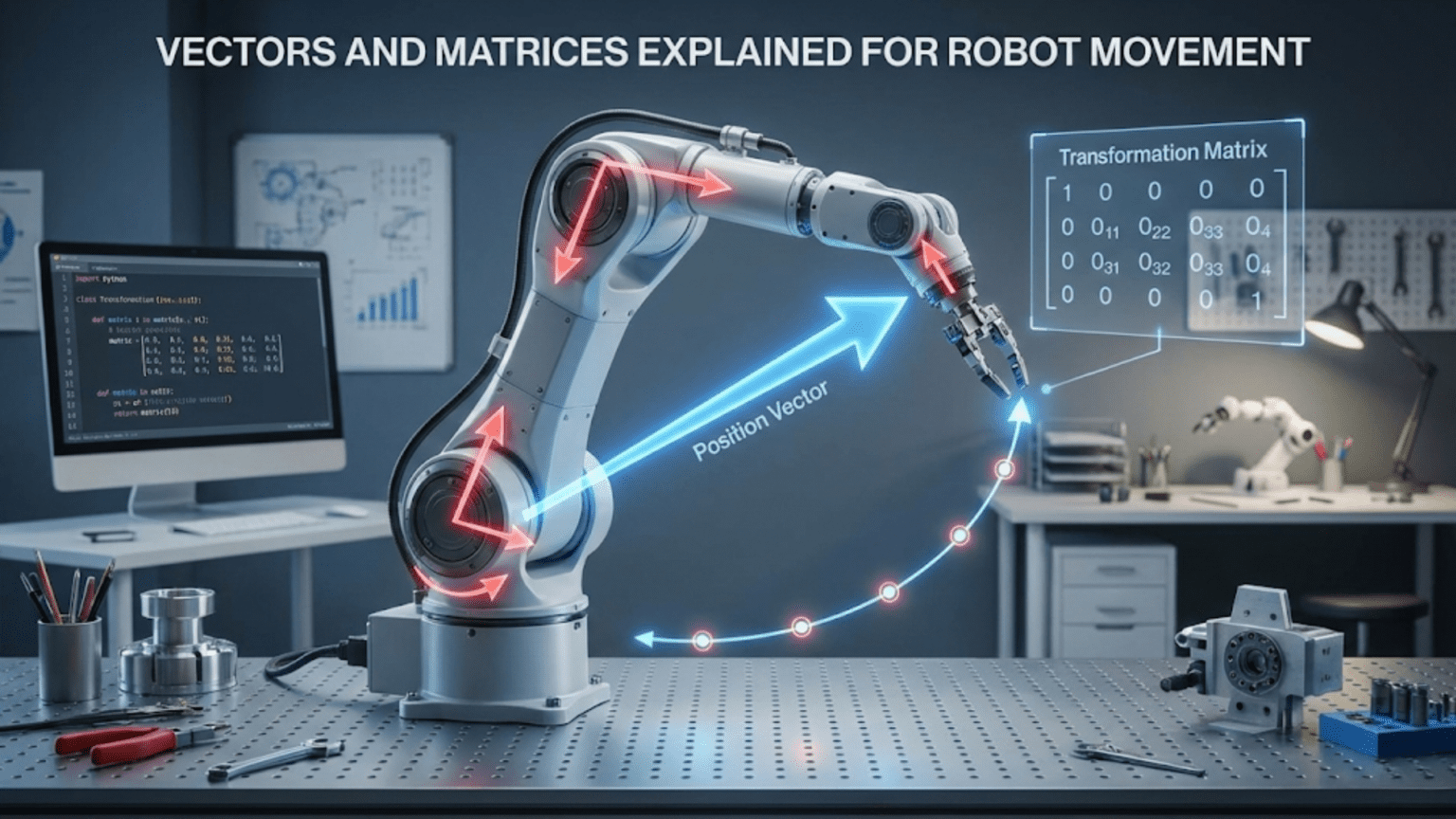
Position vectors describe locations in space relative to an origin. The position vector [3, 4] in two dimensions means “three units in the X direction and four units in the Y direction from the origin.” This vector points from the origin to the position it describes, which is why we visualize vectors as arrows. The arrow’s length represents magnitude (distance from origin), and the arrow’s direction shows which way to travel. Three-dimensional position vectors like [2, -1, 5] extend this naturally to three-dimensional space.

Displacement vectors describe movement from one position to another. If your robot starts at position [1, 2] and moves to position [4, 6], the displacement vector is [3, 4]—subtracting start position from end position gives displacement. Displacement vectors capture movement independent of absolute position. The same displacement [3, 4] applied from any starting position produces the same relative motion. This displacement property makes vectors powerful for describing movement that should work regardless of where you start.

Velocity vectors combine speed with direction of motion. A robot moving at two meters per second toward the northeast might have velocity vector [1.4, 1.4] where components represent X and Y velocity. The magnitude of the velocity vector (calculated using the Pythagorean theorem as square root of sum of squared components) gives speed. The direction of the velocity vector shows heading. Velocity vectors naturally represent the fundamental quantities needed for motion—how fast and which way.

Force vectors represent pushes and pulls on objects with magnitude and direction. A motor applying force to move a robot forward might create force vector [10, 0] in units of newtons. Multiple forces combine by vector addition—if two motors apply forces [10, 0] and [0, 5], the total force is [10, 5]. This vector addition mirrors physical intuition that forces from different directions combine to create resultant force. Understanding forces as vectors enables analyzing robot dynamics systematically.

Unit vectors have magnitude of one and indicate pure direction. The unit vector pointing in the X direction is [1, 0] in two dimensions. The unit vector pointing northeast is [0.707, 0.707] (approximately [√2/2, √2/2]). Unit vectors separate the concepts of direction from magnitude—multiply a unit vector by a scalar to get vector in that direction with desired magnitude. Normalizing any vector (dividing it by its magnitude) produces the unit vector pointing in that same direction.

Vector components break vectors into perpendicular pieces. The vector [3, 4] has X-component 3 and Y-component 4. These components tell you how much the vector extends in each axis direction. Component representation makes vectors computationally convenient—storing a few numbers completely captures all information about the vector. Operating on vectors becomes operations on their components, which computers handle efficiently through arrays of numbers.

Basic Vector Operations for Robotics

Understanding how to manipulate vectors mathematically enables calculating positions, velocities, and forces robots work with constantly. These operations follow intuitive rules matching physical intuition about motion and forces.

Vector addition combines vectors by adding corresponding components. Adding vectors [2, 3] and [1, -1] gives [3, 2]. Geometrically, vector addition chains the vectors tip-to-tail—the sum represents where you end up starting from origin, following the first vector, then following the second vector from there. For robots, vector addition combines displacements, velocities, or forces. If your robot moves displacement [2, 0] then displacement [0, 3], the total displacement is [2, 3]. Vector addition formalizes the obvious fact that separate movements combine into total movement.

Vector subtraction finds the difference between vectors by subtracting corresponding components. Subtracting [1, 1] from [4, 3] gives [3, 2]. Geometrically, the difference vector points from the tip of the second vector to the tip of the first. For robots, subtraction calculates displacement from one position to another—subtracting current position from goal position gives the vector pointing toward the goal. This operation directly answers “which direction should I move?” when you know current and target positions.

Scalar multiplication scales vectors by multiplying each component by a number. Multiplying vector [2, 3] by scalar 2 gives [4, 6]—a vector in the same direction but twice as long. Negative scalars reverse direction. Multiplying [2, 3] by -1 gives [-2, -3], pointing the opposite direction. For robots, scalar multiplication scales velocities (going twice as fast in the same direction), forces (applying more or less force in the same direction), or displacements (moving farther or less far in the same direction).

Dot product multiplies vectors to produce a scalar value measuring how aligned they are. The dot product of [3, 4] and [1, 0] is 3—computed by multiplying corresponding components and summing: 3×1 + 4×0 = 3. Geometrically, dot product equals the product of magnitudes times the cosine of angle between vectors. Dot products equal zero when vectors are perpendicular, positive when pointing generally the same direction, and negative when opposing. For robots, dot products measure alignment between directions—useful for determining whether robots are heading toward or away from targets, or whether forces oppose or assist motion.

Cross product (in three dimensions) multiplies vectors to produce a vector perpendicular to both. The cross product of [1, 0, 0] and [0, 1, 0] is [0, 0, 1]—a vector perpendicular to both inputs. Cross product magnitude equals the area of the parallelogram formed by the two vectors. For robots, cross products calculate torques from forces and lever arms, determine rotation axes, and find perpendicular directions. The right-hand rule determines cross product direction—curl right-hand fingers from first vector toward second, and thumb points in cross product direction.

Magnitude calculation finds vector length using the Pythagorean theorem. The magnitude of [3, 4] is √(3² + 4²) = 5. Magnitude tells you how far, how fast, or how strong—the scalar quantity independent of direction. For robots, magnitudes convert velocity vectors into speeds, force vectors into force magnitudes, and position vectors into distances from origin. This extraction of “how much” from directional quantities proves constantly useful.

Matrices: Transforming Vectors Systematically

While vectors represent spatial quantities, matrices provide systematic ways to transform vectors—rotating them, scaling them, or otherwise changing them according to consistent rules. Understanding matrices as transformation operators makes their abstract notation concrete.

A matrix is a rectangular array of numbers arranged in rows and columns. A 2×2 matrix has two rows and two columns, looking like:

[a  b]

[c d]

A 3×3 matrix extends to three rows and three columns. These numbers define how the matrix transforms vectors. Rather than memorizing matrix arithmetic rules, understanding that matrices encode transformations helps you grasp what matrix operations accomplish.

Matrix-vector multiplication transforms vectors according to the matrix. Multiplying a 2×2 matrix by a 2D vector produces a new 2D vector—the transformed version. The transformation applies to each vector component according to matrix entries, systematically encoding how the transformation affects different directions. This operation is what makes matrices powerful—they describe transformations that you apply by multiplying vectors by the matrix.

Rotation matrices rotate vectors without changing their length. A rotation matrix in two dimensions looks like:

[cos(θ)  -sin(θ)]

[sin(θ) cos(θ)]

where θ is the rotation angle. Multiplying any vector by this matrix rotates it by angle θ counterclockwise. For example, rotating vector [1, 0] by 90 degrees (θ = π/2) using the rotation matrix gives [0, 1]—the vector rotated from pointing right to pointing up. Rotation matrices enable robots to reason about how orientations change when rotating.

Scaling matrices change vector magnitudes. A diagonal matrix with value k on the diagonal scales all vectors by factor k. Different diagonal values scale different directions by different amounts. For example:

[2  0]
[0  3]

scales X-direction by 2 and Y-direction by 3, stretching vectors more vertically than horizontally. Robots rarely use pure scaling matrices, but understanding them helps grasp matrix transformations generally.

Identity matrix leaves vectors unchanged, analogous to multiplying by one in scalar arithmetic. The identity matrix has ones on the diagonal and zeros elsewhere:

[1  0]
[0  1]

Multiplying any vector by the identity matrix returns that same vector unchanged. Identity matrices serve as transformation “do nothing” operations and appear frequently in matrix mathematics as neutral elements.

Transformation composition through matrix multiplication combines transformations. If matrix A rotates by 45 degrees and matrix B rotates by 30 degrees, their product A×B represents rotation by 75 degrees—the combined effect of applying B then A. Matrix multiplication order matters because transformations applied in different orders produce different results. Rotating then translating differs from translating then rotating. Understanding that matrix multiplication chains transformations helps you build complex transformations from simple building blocks.

Homogeneous Coordinates: Unified Translation and Rotation

Pure rotation matrices cannot represent translation (shifting position without rotation), which robots need constantly. Homogeneous coordinates extend vectors and matrices to handle translation and rotation uniformly.

Homogeneous coordinates add an extra component to position vectors. Two-dimensional position [x, y] becomes three-dimensional homogeneous vector [x, y, 1]. Three-dimensional position [x, y, z] becomes four-dimensional homogeneous vector [x, y, z, 1]. This extra dimension seems arbitrary but enables elegant mathematics. The final component (usually 1 for positions) distinguishes positions from directions, and enables translation through matrix multiplication.

Transformation matrices in homogeneous coordinates grow to 3×3 for 2D or 4×4 for 3D. These larger matrices encode both rotation and translation. A 3×3 homogeneous transformation matrix looks like:

[R  R  tx]
[R  R  ty]
[0  0   1]

where the 2×2 R block encodes rotation, the t column encodes translation, and the bottom row remains [0, 0, 1]. This structure lets single matrix multiplication rotate and translate simultaneously—matrix-vector multiplication applies rotation through the R block and translation through the t column in one operation.

Translation in homogeneous coordinates becomes matrix multiplication rather than vector addition. To translate by [3, 2], you multiply by:

[1  0  3]
[0  1  2]
[0  0  1]

This translation matrix shifts positions by adding translation components, elegantly unified with rotation through the matrix multiplication framework. Without homogeneous coordinates, you would handle rotation through matrix multiplication and translation through vector addition—different operations requiring separate code paths. Homogeneous coordinates unify both through multiplication.

Transformation chains in homogeneous coordinates combine simply through matrix multiplication. A transformation rotating then translating can represent as single matrix by multiplying the rotation matrix by the translation matrix. This composition extends to arbitrary chains—rotation, translation, rotation, translation, etc.—all composing through matrix multiplication. Chaining transformations through multiplication dramatically simplifies the mathematics of coordinate frame transformations that robots require constantly.

Inverse transformations in homogeneous coordinates use matrix inversion. If matrix M transforms from frame A to frame B, the inverse matrix M⁻¹ transforms from frame B to frame A. Libraries compute matrix inverses, enabling bidirectional transformations between coordinate frames. This inversion capability proves essential when you receive information in one frame but need it in another—you apply the inverse transformation to convert back.

Practical Robot Applications of Vector-Matrix Mathematics

These abstract mathematical objects prove their worth through practical robot applications where vector-matrix operations directly solve real problems.

Dead reckoning navigation integrates velocity vectors over time to estimate position. If your robot moves with velocity [1, 0.5] for two seconds, it displaces by 2×[1, 0.5] = [2, 1]. Repeatedly adding these displacement vectors to current position tracks where the robot has moved. This integration of velocity to position uses vector scaling and addition naturally. While dead reckoning accumulates errors over time, the basic position tracking through vector operations provides starting point for more sophisticated navigation.

Robot arm forward kinematics chains transformation matrices from base through each joint to calculate end-effector position. Each joint contributes transformation matrix encoding its rotation and its spatial relationship to the next joint. Multiplying all these matrices produces single transformation from base to end-effector. This matrix chain multiplication elegantly handles arbitrarily complex arm configurations—six-degree-of-freedom arms use six transformation matrices multiplied together. The mathematics scales naturally to any number of joints.

Inverse kinematics for simple arms uses vector-matrix operations to solve for joint angles. For two-joint planar arms, the problem reduces to solving systems of equations derived from transformation matrices. While complex arms require numerical methods, understanding that the problem formulates as finding joint angles that produce desired transformation matrix from base to end-effector shows how vector-matrix mathematics frames the inverse kinematics problem.

Path planning in configuration space represents robot states as vectors and obstacle boundaries as vectors in high-dimensional space. A robot arm with six joints has six-dimensional configuration vector specifying all joint angles. Path planning searches this configuration space for collision-free paths from start to goal configuration vectors. Vector distances measure configuration similarity, and vector interpolation generates intermediate configurations between waypoints. This representation of robot states as vectors in configuration space enables powerful path planning algorithms.

Sensor fusion combines measurements from multiple sensors through weighted vector addition or matrix operations. If two sensors estimate robot position with different uncertainties, fusing measurements weights each estimate inversely proportional to its uncertainty. Kalman filtering implements optimal sensor fusion through matrix operations that statistically combine measurements with motion predictions. Understanding sensor fusion fundamentally uses vector-matrix mathematics to combine multiple imperfect measurements into better estimates.

Force control for compliant manipulation calculates required motor torques from desired forces through matrix transformations. The robot’s Jacobian matrix (describing how joint velocities relate to end-effector velocity) transforms desired end-effector forces into required joint torques. Implementing force control that makes robots safely interact with environments requires these matrix transformations converting between force domains and torque domains. The mathematics enables compliant behaviors that pure position control cannot achieve.

Visualizing Vector-Matrix Operations

Abstract notation hides the geometric meaning of vector-matrix mathematics. Developing visual intuition about what operations do geometrically makes mathematics meaningful and memorable.

Vectors as arrows from origin to point provide concrete visualization. When you see notation [3, 4], visualize an arrow starting at origin extending three units right and four units up. This arrow representation makes vector addition obvious—chaining arrows tip-to-tail shows how movements combine. Vector subtraction reverses the second arrow. Scalar multiplication stretches or shrinks the arrow. These geometric interpretations make symbolic operations intuitive.

Matrix transformations as deformations of the coordinate grid visualize what matrices do to space. Draw a grid of points, then transform every point by multiplying by the transformation matrix. Rotation matrices rotate the entire grid. Scaling matrices stretch the grid. Shear matrices distort the grid into parallelograms. Visualizing how matrices transform the grid shows their action on all vectors simultaneously—the grid deformation characterizes the transformation.

Unit vectors transformed by matrices show how matrices affect different directions. Take the unit vector pointing right [1, 0] and left [0, 1]. Transform both by your matrix. Where these unit vectors end up after transformation shows how the matrix affects X and Y directions respectively. This provides intuitive understanding—if transformed unit vectors remain perpendicular with equal length, the matrix is pure rotation. If they change length differently, the matrix includes scaling.

Determinants visualize as area scaling factors. The determinant of a 2×2 matrix tells you how much that transformation scales areas. A transformation with determinant 2 doubles all areas. Determinant -2 doubles areas and flips orientation (reflected). Zero determinant means the transformation collapses space to lower dimension. For robotics, determinants indicate whether transformations preserve volumes (important for singularity checking) and whether they are invertible (determinant ≠ 0 means inverse exists).

Eigenvalues and eigenvectors show special directions that matrices merely scale. If vector v is an eigenvector of matrix M, then M×v = λv for some scalar λ (the eigenvalue). The matrix scales the eigenvector but does not change its direction. While computing eigenvalues requires linear algebra algorithms, understanding that they represent special invariant directions helps interpret control system behavior and stability analysis. Eigenvalues determine whether control systems converge or oscillate.

Common Vector-Matrix Mistakes in Robotics

Understanding frequent errors helps you avoid frustration and debug problems when vector-matrix operations produce unexpected results.

Dimension mismatch errors occur when attempting operations on incompatible vector or matrix sizes. You cannot add 2D vector to 3D vector. You cannot multiply 2×3 matrix by 2D vector (needs 3D vector). Tracking dimensions carefully and ensuring compatible sizes prevents these errors. Modern programming languages with type systems can catch dimension mismatches at compile time, but manual dimension tracking prevents errors when using dynamically-typed languages.

Row vectors versus column vectors cause subtle bugs when code expects one but receives the other. Mathematical convention typically treats vectors as column vectors (nx1 matrices), but some programming environments default to row vectors (1xn matrices). Matrix multiplication cares about this distinction—multiplying matrix by column vector differs from multiplying row vector by matrix. Maintaining consistent vector conventions throughout code prevents frustrating debugging sessions.

Matrix multiplication order errors produce wrong results because matrix multiplication is not commutative—A×B usually differs from B×A. Transformation composition particularly suffers from order errors. Rotating then translating produces different result than translating then rotating. Carefully tracking what transformation order you intend and ensuring matrix multiplication matches prevents these errors. Drawing diagrams showing desired transformation sequence helps verify correct multiplication order.

Using wrong transformation direction applies forward transformation when you need inverse or vice versa. If you need to transform from frame A to frame B but apply transformation from B to A, results are completely wrong. Clearly labeling transformations with source and destination frames helps prevent using inverses when forward transformations are needed. Drawing frame relationship diagrams clarifies which transformation direction is needed.

Forgetting to normalize vectors causes magnitude errors. If you use vector as direction but forget to normalize it, any magnitude in the original vector affects calculations incorrectly. Always normalize vectors when you care about direction independent of magnitude. Unit vectors eliminate magnitude as confounding factor, making direction-dependent calculations correct.

Mixing homogeneous and non-homogeneous coordinates creates mysterious bugs. If you multiply 3×3 homogeneous transformation matrix by 2D non-homogeneous vector, dimensions match but semantics are wrong. The transformation treats the vector incorrectly. Consistently using homogeneous or non-homogeneous coordinates throughout calculations prevents these subtle errors.

Learning Vector-Matrix Mathematics Practically

Rather than comprehensive linear algebra course, targeted learning focused on robotics applications teaches what you need more efficiently.

Start with geometric intuition before symbolic manipulation. Draw vectors as arrows. Visualize rotations as turning the coordinate grid. Build physical understanding of what operations accomplish geometrically before worrying about computational procedures. This intuition makes subsequent symbolic mathematics meaningful rather than arbitrary manipulation rules.

Implement operations in code to develop computational understanding. Write functions that multiply matrices, rotate vectors, and chain transformations. Implementing these operations yourself (even if you later use library implementations) builds deep understanding of what calculations actually do. When your code produces correct behavior, you know your understanding works.

Use robotics examples as learning motivation. Rather than abstract linear algebra problems, study how robot arms use transformation matrices or how mobile robots use velocity vectors. The concrete robotics context makes mathematics purposeful and memorable. You remember that matrix multiplication chains transformations because you understand why robots need chained transformations.

Leverage libraries for practical work while understanding underlying mathematics. NumPy in Python, Eigen in C++, or similar libraries implement vector-matrix operations efficiently. Use these libraries for real projects while maintaining conceptual understanding of what operations do. You need not manually multiply 4×4 matrices, but you should understand that multiplication combines transformations.

Verify calculations with simple test cases. When implementing transformation, test with unit vectors you can calculate by hand. Does rotating [1, 0] by 90 degrees give [0, 1]? Does translating by [2, 3] move points correctly? These sanity checks catch implementation errors before they cause problems in real applications.

Build intuition gradually through repeated application. Linear algebra mastery develops through encountering concepts repeatedly in different robotics contexts. Each application deepens understanding. Initially confusing concepts become intuitive through experience. This gradual building through practice works better than attempting complete understanding before application.

Vector-Matrix Mathematics as Robot Movement Language

Vectors and matrices form the natural mathematical language for describing robot motion, orientation, and spatial relationships. They directly represent physical quantities robots manipulate—positions, velocities, forces, and transformations. This natural correspondence between mathematics and physical reality makes vectors and matrices powerful rather than arbitrary abstractions.

Your journey to vector-matrix fluency begins with geometric visualization—seeing vectors as arrows and matrices as transformations. Building on this intuition, symbolic notation becomes meaningful rather than mystical. Through practical application in robotics projects, initially confusing operations become tools you use naturally. The mathematics that seemed intimidating proves remarkably intuitive when understood through spatial geometry and robotics applications.

Every robot you build uses vector-matrix mathematics whether or not you recognize it. Motion planning manipulates position vectors. Coordinate transformations multiply transformation matrices. Sensor fusion combines measurement vectors. Understanding this underlying mathematics changes you from blindly following formulas to deliberately choosing mathematical operations that accomplish what your robot needs. This transformation from passive mathematics consumer to active mathematics user dramatically expands what robots you can design and what behaviors you can implement.

Start applying vector-matrix thinking in your next robotics project. Explicitly represent positions as vectors. Think about transformations as matrices. When your robot needs to combine motions or transform between coordinate frames, consciously apply vector addition or matrix multiplication rather than ad-hoc arithmetic. Through deliberate practice using these mathematical structures, vectors and matrices become natural tools in your robotics toolkit—mathematical language you speak fluently when reasoning about how robots move through and interact with spatial environments.