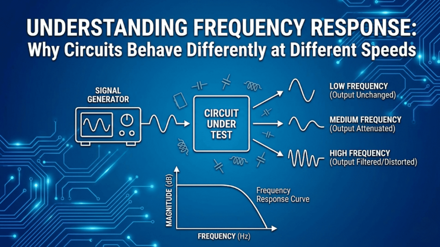
Frequency response describes how a circuit’s output amplitude and phase change as the frequency of the input signal varies. Circuits behave differently at different frequencies because capacitors and inductors have impedances that change with frequency—capacitors pass high frequencies easily but block low ones, while inductors pass low frequencies but block high ones. This frequency-dependent behavior is what makes filters possible: an RC low-pass filter passes audio but blocks radio frequencies; a tuned LC circuit passes only a narrow band of frequencies for a radio station; an amplifier’s gain drops above its bandwidth frequency. Every real circuit has a characteristic frequency response that defines which frequencies it amplifies, passes, attenuates, or blocks.
Introduction: The Frequency Dimension of Electronics
Most beginner electronics focuses on what happens at a single moment in time or at a single frequency—measuring DC voltages, calculating resistor values, determining LED current. But real electronic signals are not single-frequency tones or steady DC levels. A human voice contains frequencies from 80Hz to 8kHz. A digital data stream at 100Mbps contains frequency components from DC to several hundred megahertz. A radio signal occupies a specific narrow band of the radio spectrum. Background electrical noise spans a broad spectrum from DC to gigahertz.
Every real circuit processes signals containing a range of frequencies. And here is the fundamental insight that makes frequency response important: no real circuit treats all frequencies identically. Every circuit has a characteristic behavior across frequency—some frequencies pass easily, others are attenuated or blocked entirely, and the phase relationship between input and output varies with frequency.
This frequency-varying behavior is not a flaw to be worked around—it is the mechanism that makes the vast majority of useful electronic functions possible. Without it, we could not filter noise from signals, separate one radio station from another, equalize audio to compensate for speaker characteristics, prevent aliasing in analog-to-digital converters, stabilize feedback amplifiers, or transmit digital data reliably at high speeds.
Understanding frequency response means understanding the frequency dimension of electronics—the axis along which circuits express their most characteristic behaviors, the domain in which design decisions about capacitors and inductors and circuit topology play out in observable, measurable ways. With this understanding, a schematic stops being a collection of static connections and becomes a description of a system with a rich, purposeful behavior that unfolds across frequency.
This article builds frequency response understanding from the ground up. We’ll see why different frequencies behave differently through the lens of impedance, learn to visualize frequency response through Bode plots, explore the major filter types and their applications, understand bandwidth and how it limits circuit performance, and connect frequency response to the practical circuits you build and use.
Why Frequency Matters: Impedance Revisited
The Root Cause
As established in the impedance article, capacitors and inductors have impedances that change with frequency:
Capacitive reactance: X_C = 1/(2πfC)
- Falls with increasing frequency
- At low f: high impedance (blocks current)
- At high f: low impedance (passes current freely)
Inductive reactance: X_L = 2πfL
- Rises with increasing frequency
- At low f: low impedance (passes current freely)
- At high f: high impedance (blocks current)
These frequency-dependent impedances interact with resistors (frequency-independent) in voltage divider relationships. Since a voltage divider’s output ratio depends on the impedances involved, and at least one impedance changes with frequency, the output ratio changes with frequency—and so does the phase relationship.
This is the root cause of all frequency response: reactive components have frequency-dependent impedances that create frequency-dependent voltage dividers.
The RC Voltage Divider at Different Frequencies
The simplest demonstration is a series RC circuit with the output taken across the capacitor:
Input ──[R]──┬── Output
             │
            [C]
             │
GNDOutput voltage ratio: V_out/V_in = X_C / √(R² + X_C²) = 1 / √(1 + (2πfRC)²)
At very low frequency (f → 0): X_C → ∞, so X_C >> R V_out/V_in → 1 (full input appears at output)
At the cutoff frequency (f_c = 1/2πRC, where X_C = R): V_out/V_in = 1/√(1 + 1) = 1/√2 ≈ 0.707 (-3dB)
At very high frequency (f → ∞): X_C → 0, so X_C << R V_out/V_in → 0 (output disappears)
This is a low-pass filter—low frequencies pass, high frequencies are attenuated. The circuit “responds” differently to different frequencies, and this characteristic behavior is its frequency response.
Bode Plots: Visualizing Frequency Response
What Is a Bode Plot?
A Bode plot (named after Hendrik Bode, Bell Labs engineer) is a standard two-graph representation of frequency response:
Upper graph (magnitude/gain):
- Horizontal axis: Frequency on a logarithmic scale (decades: 10Hz, 100Hz, 1kHz, 10kHz…)
- Vertical axis: Gain in decibels (dB = 20 × log₁₀(V_out/V_in))
Lower graph (phase):
- Horizontal axis: Same frequency scale
- Vertical axis: Phase shift in degrees (from -180° to +180°)
Why Logarithmic Frequency Scale?
Electronic circuits operate across enormous frequency ranges—from 0.001Hz (very slow biomedical signals) to 100GHz (millimeter wave radar). A linear frequency scale would compress all interesting low-frequency behavior into a tiny region while most of the axis shows “nothing happening” at higher frequencies.
A logarithmic scale solves this by allocating equal space to each decade (factor of 10) of frequency. Each decade looks the same width on the axis, regardless of whether it’s 10–100Hz or 10MHz–100MHz.
Why dB for Gain?
Decibels compress enormous gain ranges (0.001 to 1,000,000) into manageable numbers (-60dB to +120dB). They also make cascaded stages easy—stages in series have gains that multiply as ratios but add in dB.
Key dB reference points:
- 0 dB: Gain = 1 (input equals output)
- +3 dB: Gain = √2 ≈ 1.414 (output 41% larger)
- -3 dB: Gain = 1/√2 ≈ 0.707 (output 29% smaller, power halved)
- +20 dB: Gain = 10
- -20 dB: Gain = 0.1
- +40 dB: Gain = 100
- -40 dB: Gain = 0.01
- -60 dB: Gain = 0.001
Reading a Bode Plot: RC Low-Pass Filter Example
For a simple RC low-pass filter with R = 10kΩ, C = 10nF: f_c = 1/(2π × 10,000 × 10×10⁻⁹) = 1,592Hz ≈ 1.6kHz
Magnitude plot behavior:
- Below 160Hz (one decade below f_c): Gain ≈ 0 dB (flat, passes freely)
- At 1.6kHz (f_c): Gain = -3 dB (output at 70.7% of input)
- Above 16kHz (one decade above f_c): Gain ≈ -20 dB (output at 10% of input)
- Each decade above f_c: Additional -20 dB attenuation
- Slope above f_c: -20 dB/decade (or equivalently -6 dB/octave)
Phase plot behavior:
- Well below f_c: Phase ≈ 0° (in phase)
- At f_c: Phase = -45° (current leads voltage by 45°)
- Well above f_c: Phase → -90° (maximum lag)
The asymptotic Bode approximation: Real Bode plots have smooth curves, but engineers often use straight-line approximations:
- Flat at 0 dB below f_c
- Drops at -20 dB/decade starting at f_c
- Phase transitions from 0° to -90° centered at f_c, spanning from f_c/10 to 10×f_c
These approximations are accurate within ±3 dB everywhere and within ±6° on phase—sufficient for most design work.
-3 dB Bandwidth: The Standard Definition
The bandwidth of a circuit (amplifier, filter, etc.) is defined as the frequency range over which gain stays within -3 dB of its maximum value.
For a low-pass filter: bandwidth = f_c (0Hz to cutoff frequency) For an amplifier: bandwidth = f_H – f_L (between upper and lower -3 dB frequencies) For a band-pass filter: bandwidth = f_H – f_L (between the two -3 dB frequencies)
Why -3 dB as the standard? At -3 dB, power is halved (since P ∝ V², and V is at 1/√2 = 0.707). This is a natural, physically meaningful threshold—below it, the circuit is “significantly” attenuating the signal.
The Four Fundamental Filter Types
Low-Pass Filter
Passes: Frequencies below the cutoff frequency Attenuates: Frequencies above the cutoff frequency Slope above cutoff: -20 dB/decade per pole (RC stage)
Simple RC low-pass:
Input ──[R]──┬── Output
             │
            [C]
             │
GNDf_c = 1/(2πRC)
Applications:
- Anti-aliasing filter: Before an ADC, removes frequencies above half the sampling rate to prevent aliasing artifacts
- Audio tone control (bass): Passes bass frequencies; reference for boosting/cutting
- Power supply filtering: Passes DC, attenuates ripple and noise
- Smoothing PWM output: Converts PWM square wave to analog voltage
- Noise reduction: Removes high-frequency noise from slow signals
Higher-order low-pass: Multiple RC stages (or LC stages) cascade to create steeper rolloff:
- 1st order (1 RC): -20 dB/decade
- 2nd order (2 RC, or 1 LC): -40 dB/decade
- 4th order: -80 dB/decade
Each added pole adds another -20 dB/decade to the rolloff slope above cutoff.
High-Pass Filter
Passes: Frequencies above the cutoff frequency Attenuates: Frequencies below the cutoff frequency Slope below cutoff: +20 dB/decade per pole (rises toward f_c)
Simple RC high-pass:
Input ──[C]──┬── Output
             │
            [R]
             │
GNDf_c = 1/(2πRC)
Applications:
- DC blocking / AC coupling: The classic use—capacitor in series with signal path removes DC bias while passing AC signal
- Audio tone control (treble): Passes treble frequencies
- Differentiation (approximate): Output proportional to rate of change of input (below f_c)
- Subsonic filter: Removes infrasonic rumble below 20Hz from audio before amplification
- Removing low-frequency drift: Sensor drift is often slower than the signal of interest; high-pass filter removes it
Band-Pass Filter
Passes: Frequencies within a defined band (between f_L and f_H) Attenuates: Frequencies both below f_L and above f_H Center frequency: f_0 = √(f_L × f_H) Bandwidth: BW = f_H – f_L
Simple RLC band-pass (series resonant): At resonance, X_L = X_C, net reactance = 0, impedance = R only—maximum current, maximum output.
Quality factor Q: Q = f_0 / BW = f_0 / (f_H – f_L)
Higher Q = narrower bandwidth = more selective filter
Applications:
- Radio tuning: Selects one station from the broadcast band (very high Q required—crystal filters achieve Q of tens of thousands)
- Audio graphic equalizer: Each band controlled by a band-pass filter centered at a specific audio frequency
- Intermediate frequency (IF) filter: Fixed band-pass filter in superheterodyne radio receivers
- Touch-tone telephone decoder (DTMF): Bank of band-pass filters detecting specific tone pairs
Band-Stop (Notch) Filter
Passes: All frequencies except those within a defined band Attenuates: Frequencies within the stop band
Special case — notch filter: Extremely narrow band-stop at a specific frequency.
Applications:
- 60Hz/50Hz notch filter: Removes power line hum from audio and medical signals (ECG, EEG)
- Interference rejection: Removes a specific interference frequency while preserving signal
- Feedback suppression in PA systems: Notches out the feedback frequency that causes howling
Amplifier Frequency Response
Why Amplifiers Have Bandwidth Limits
Every amplifier has a frequency range over which it provides its intended gain—the bandwidth. Outside this range, gain falls off. This limitation exists because:
Internal capacitances: Every transistor has parasitic capacitances between its terminals (junction capacitances for BJTs, gate capacitances for MOSFETs). At high frequencies, these capacitances provide low-impedance paths that bypass the signal, reducing gain.
Feedback network frequency response: Op-amps and transistor amplifiers with feedback have frequency responses determined by the interaction of gain and feedback—stability requirements limit bandwidth.
Miller effect: In an inverting amplifier, capacitance between output and input is multiplied by the gain factor (Miller multiplication), creating an effectively larger input capacitance that limits bandwidth.
The Gain-Bandwidth Product (GBW)
For most amplifier topologies:
Gain × Bandwidth = Constant (GBW or GBP)
If you need more gain, you sacrifice bandwidth. If you need more bandwidth, you must accept lower gain.
Example — op-amp with GBW = 1MHz:
- At unity gain (1×): Bandwidth = 1MHz
- At 10× gain: Bandwidth = 100kHz
- At 100× gain: Bandwidth = 10kHz
- At 1000× gain: Bandwidth = 1kHz
Practical implication: A single op-amp stage with GBW = 1MHz cannot amplify 10kHz audio signals with gain > 100. If 1000× gain is needed across audio bandwidth (20kHz), GBW must be at least 1000 × 20kHz = 20MHz.
This is why cascading two stages of 30× gain (GBW requirements much lower per stage) often outperforms one stage of 900× gain.
Phase Margin and Stability
Amplifiers with negative feedback (all op-amp circuits, most practical transistor amplifiers) can become unstable if the feedback becomes positive at some frequency—causing oscillation.
Phase margin: The difference between the phase at the frequency where gain = 1 (unity gain crossing) and -180°.
- Phase margin > 45°: Stable, minimal ringing
- Phase margin 20°–45°: Marginal stability, some ringing
- Phase margin < 20°: Risk of oscillation
Frequency compensation (adding capacitors to deliberately roll off gain at high frequencies) is used to ensure adequate phase margin. This is why op-amps have a dominant pole compensating capacitor (built-in for most) that limits their unity-gain bandwidth.
Frequency Response in Real Systems
Audio Systems: The Audible Spectrum
Human hearing spans approximately 20Hz to 20kHz. Audio system design revolves around:
Flat frequency response (ideal): The same output amplitude for every frequency within 20–20kHz. A “ruler-flat” response means no coloration—the system reproduces exactly what was recorded.
Frequency response specification: Stated as ±dB over a frequency range. “20Hz–20kHz ±0.5dB” means the response varies by no more than ±0.5dB across the audio band — very flat.
Real-world deviations:
- Microphones roll off at low and high frequency extremes
- Speakers have resonance peaks and roll-offs
- Room acoustics create complex frequency response variations
- Equalizers deliberately alter frequency response to compensate
Digital Systems: Bandwidth and Signal Integrity
Digital signals appear to be binary (HIGH/LOW), but they contain analog frequency components. A square wave with period T has fundamental frequency f = 1/T plus harmonics at 3f, 5f, 7f… (odd harmonics only for a perfect square wave).
Rise time and bandwidth relationship: For a circuit with bandwidth BW (-3dB), the rise time of a step response is approximately: t_rise ≈ 0.35 / BW
Example: A 100MHz bandwidth oscilloscope measures rise times as fast as: t_rise = 0.35 / 100MHz = 3.5ns
Why digital design needs frequency response thinking: A 1Gbps serial data signal has a bit period of 1ns. Its highest significant frequency components reach several hundred MHz to several GHz. PCB traces, connectors, and IC packages must have sufficient bandwidth to pass these frequency components without attenuation—otherwise edges become rounded, timing margins shrink, and data errors occur.
This is why high-speed digital design (PCIe, DDR memory, high-speed USB) requires the same impedance and frequency response analysis as RF circuit design.
RF Systems: Selectivity and Bandwidth
Radio receivers must:
- Select one signal from among thousands in the radio spectrum (high selectivity = narrow bandwidth at the desired frequency)
- Reject all other signals
- Amplify the selected signal without distortion
Superheterodyne receiver frequency response: The radio frequency selectivity is provided by bandpass filters centered at an intermediate frequency (IF)—typically 455kHz for AM, 10.7MHz for FM. By converting all incoming signals to the same IF frequency (through mixing), a single, carefully designed IF filter provides consistent selectivity regardless of the tuned frequency.
The IF filter’s frequency response—its bandwidth and shape—determines the receiver’s channel selectivity.
Control Systems: The Crossover Frequency
In feedback control systems (motor controllers, temperature regulators, power supply feedback loops), the frequency response determines stability and response speed.
Loop gain: The total gain around the feedback loop. Crossover frequency (f_c): The frequency where loop gain = 1 (0 dB). Phase margin: How much phase is left before the feedback becomes positive (destabilizing) at f_c.
Voltage regulators, motor speed controllers, and operational amplifiers all have designed frequency responses that balance speed of response against stability. A faster response (higher crossover frequency) requires more careful phase compensation.
Measuring and Analyzing Frequency Response
The Swept-Frequency Method
The classical approach to measuring frequency response:
- Apply a sine wave at frequency f₁ to the circuit input
- Measure input and output amplitudes and phase difference
- Calculate gain = V_out/V_in in dB and phase shift
- Repeat at f₂, f₃… across the range of interest
- Plot the results on a Bode-style graph
Modern spectrum analyzers and network analyzers automate this process, sweeping across thousands of frequency points and plotting the complete Bode diagram in seconds.
The Impulse/Step Response Method
Any linear circuit’s frequency response can be mathematically derived from its step response (how it responds to a sudden voltage step):
- A circuit that responds slowly to a step has a narrow bandwidth
- The step response rise time relates to bandwidth: BW ≈ 0.35/t_rise
- The Fourier transform of the step response gives the frequency response
This is why oscilloscopes with sufficient bandwidth can verify the frequency response of amplifiers by measuring step response.
FFT (Fast Fourier Transform) Analysis
An oscilloscope with FFT capability or a spectrum analyzer can decompose any signal into its frequency components—showing what frequencies are present and at what amplitudes. This is invaluable for:
- Identifying harmonic distortion in amplifiers (components at 2f, 3f above the fundamental)
- Finding interference sources (unexpected spectral peaks)
- Verifying filter performance (measuring actual attenuation vs. frequency)
- Characterizing oscillator spectral purity
Comparison Table: Filter Types at a Glance
| Property | Low-Pass | High-Pass | Band-Pass | Band-Stop/Notch |
|---|---|---|---|---|
| Passes | f < f_c | f > f_c | f_L < f < f_H | f < f_L and f > f_H |
| Attenuates | f > f_c | f < f_c | f outside band | f_L < f < f_H |
| Key parameter | Cutoff f_c | Cutoff f_c | Center f₀, Q | Notch f₀, Q |
| Rolloff slope (1st order) | -20 dB/dec above f_c | +20 dB/dec below f_c | ±20 dB/dec outside band | Varies |
| Phase at f_c | -45° | +45° | 0° (in-band) | ±90° (at f₀) |
| Simplest implementation | RC (R series, C shunt) | RC (C series, R shunt) | RLC series/parallel | Twin-T, Wien, RLC |
| Common applications | Anti-aliasing, smoothing, noise | DC blocking, AC coupling | Radio tuning, EQ band | Hum removal, interference |
| Audio application | Bass tone control, rumble filter | Treble boost, subsonic filter | Graphic EQ, parametric EQ | 60Hz notch filter |
| Power application | EMI filter output | N/A | N/A | Power line notch |
Practical Design Guidance
Designing for a Specific Cutoff Frequency
RC filter cutoff frequency: f_c = 1/(2πRC)
Choosing R and C:
- Choose C from standard values (consider what’s in stock): e.g., C = 10nF
- Calculate R: R = 1/(2π × f_c × C)
- Round R to nearest standard value and recalculate actual f_c
Example: 1kHz low-pass for audio Choose C = 10nF R = 1/(2π × 1000 × 10×10⁻⁹) = 15,915Ω → Use 15kΩ (standard) Actual f_c = 1/(2π × 15,000 × 10×10⁻⁹) = 1,061Hz ≈ 1.06kHz ✓
When to Use Active vs. Passive Filters
Passive filters (R, L, C only):
- No power supply needed
- Cannot provide gain (only attenuation)
- Inductor-based filters can be bulky at audio frequencies
- Suitable for RF, power line filtering, simple signal conditioning
Active filters (op-amp + R + C):
- Can provide gain along with filtering
- No inductors needed (replaced by op-amp feedback)
- Limited to frequency range below op-amp bandwidth
- Preferred for audio and instrumentation frequencies
- Easier to cascade for higher-order response
For audio (20Hz–20kHz): Active filters preferred (inductor values for passive would be very large) For RF (MHz–GHz): Passive LC filters required (op-amps too slow) For EMI filtering: Passive LC preferred (must handle large power)
Common Frequency Response Problems and Solutions
Problem: Circuit oscillates at an unexpected high frequency Diagnosis: Insufficient phase margin in feedback loop; gain too high at the phase inversion frequency Solution: Add compensation capacitor to roll off gain before phase crosses -180°; reduce gain; add series resistor to op-amp output
Problem: Audio amplifier sounds “dull” (lacks treble) Diagnosis: Bandwidth limitation; stray capacitance forming low-pass filter; gain-bandwidth limit of amplifier Solution: Reduce circuit capacitance; use wider-bandwidth amplifier; reduce gain per stage
Problem: Switching power supply output has audible whine Diagnosis: Switching frequency or harmonics within audio band; insufficient filtering Solution: Increase switching frequency above 20kHz; improve LC output filter; add ferrite bead at output
Problem: Sensor reading drifts slowly with temperature Diagnosis: Low-frequency variation is slower than signal of interest Solution: Add high-pass filter with cutoff below signal frequency but above drift frequency
Conclusion: Frequency as the Master Variable
Frequency response is not an advanced specialty—it is a fundamental dimension of all electronic circuit behavior. Every component, every trace, every circuit topology has a characteristic frequency response, and understanding this response is what separates circuits that work predictably from circuits that work only by accident.
The Core Insights
Reactive components create frequency-dependent behavior. Capacitors and inductors have impedances that change with frequency. This creates frequency-dependent voltage dividers—the root cause of all filter behavior.
Filters are purposeful frequency response. Low-pass, high-pass, band-pass, and band-stop filters are simply circuits whose frequency response is engineered to pass some frequencies and reject others. Every filter design is a frequency response design.
Amplifiers have limited bandwidth. Real amplifiers cannot amplify all frequencies equally. The gain-bandwidth product sets a fundamental limit; designing for required bandwidth at required gain is a core amplifier design challenge.
Phase response matters as much as gain. The phase relationship between input and output changes with frequency. In audio, phase errors cause subtle coloration. In feedback systems, phase errors cause instability and oscillation.
Digital signals live in the frequency domain too. High-speed digital design requires the same frequency response thinking as analog and RF design. The “frequency content” of digital signals determines what bandwidth a trace, connector, or IC must support.
The Practical Payoff
With frequency response understanding:
- You know why that capacitor was placed where it was
- You can predict whether a filter will solve your noise problem
- You can understand why an op-amp circuit oscillates and how to fix it
- You can design RC, LC, and active filters to specification
- You can read an amplifier datasheet’s frequency response plot and extract meaningful design information
- You can interpret oscilloscope FFT displays to diagnose circuit problems
The frequency axis is where circuits reveal their true character. Learning to read, predict, and design frequency response is learning to work with circuits on their own terms—in the domain where their behavior is richest, most useful, and most instructive.