Introduction
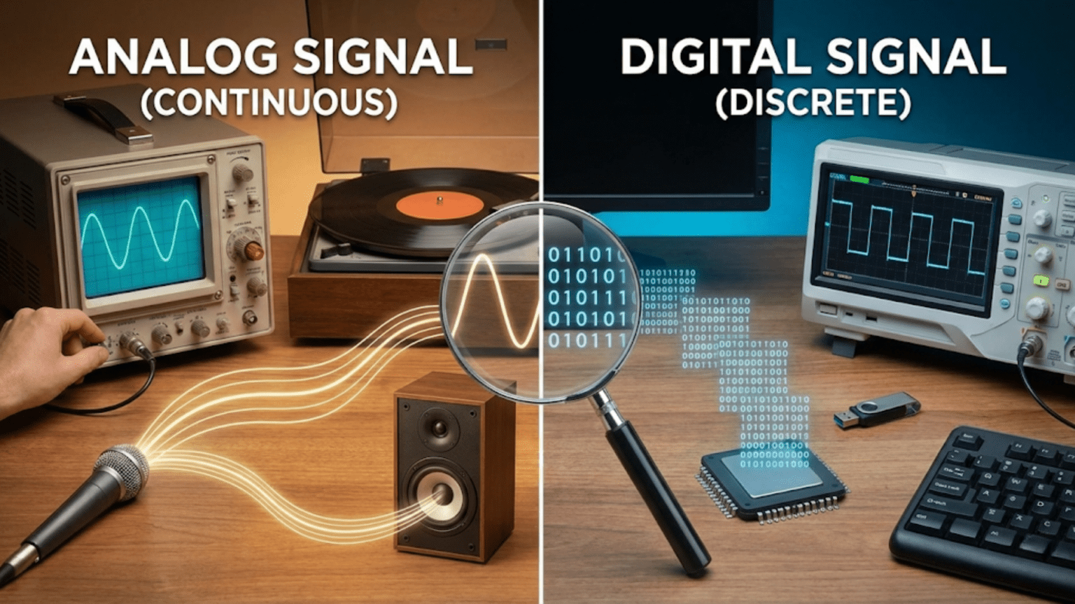
The distinction between analog and digital signals represents one of the most fundamental conceptual divides in electronics, separating continuous smoothly-varying signals that can take any value within a range from discrete stepped signals that exist only at specific predetermined levels. This analog-digital distinction affects everything from how information is represented and processed through how circuits are designed and how signals resist noise and degradation, with the shift from analog to digital technologies over recent decades transforming electronics from devices requiring careful calibration and suffering from cumulative noise and drift into robust systems that process information reliably despite imperfect components and noisy environments. Understanding the fundamental differences between these two signal types provides essential context for comprehending modern electronics and appreciating why digital technology has come to dominate applications from audio and video through telecommunications to computing and control systems.
For beginners encountering analog and digital concepts, the terminology might initially feel abstract because signals themselves are invisible electrical phenomena that cannot be directly observed without measurement instruments. Yet the analog-digital distinction maps naturally to everyday experiences that make these concepts concrete and intuitive. An analog thermometer with a continuously moving needle that can point to any temperature smoothly represents analog operation, while a digital thermometer displaying distinct numerical values like seventy-two point three degrees represents digital operation. The analog needle can indicate seventy-two point two five degrees or seventy-two point two seven degrees or any intermediate value, while the digital display jumps from seventy-two point three directly to seventy-two point four without ever showing intermediate values, illustrating the continuous nature of analog representation versus the discrete stepped nature of digital representation.
The practical implications of analog versus digital signal types affect how circuits process information and how robust that processing is against noise and imperfections. Analog circuits manipulate continuously variable voltages and currents through components like resistors, capacitors, and transistors operating in linear regions where output varies smoothly with input. These circuits provide elegant simplicity and immediate response but suffer from cumulative noise where each processing stage adds distortion and drift, with signal quality degrading as information passes through multiple analog stages. Digital circuits treat signals as binary values representing zeros and ones, processing information through logic gates that regenerate clean transitions at each stage. This regeneration prevents cumulative noise accumulation, allowing digital signals to pass through unlimited processing stages without degradation as long as noise remains below thresholds that would flip bits incorrectly.
The historical evolution from analog to digital electronics reveals both the advantages digital technology provides and the contexts where analog processing remains preferable or necessary. Early electronics relied entirely on analog techniques because digital processing requires fast switching devices and complex circuitry that vacuum tubes and early transistors could not efficiently provide. The development of integrated circuits enabled practical digital electronics, with increasing integration density making digital signal processing increasingly cost-effective compared to analog alternatives. Today, most information processing occurs digitally even when signals originate as analog phenomena from the physical world, with analog-to-digital converters transforming sensor outputs into digital form for processing, storage, and transmission using digital techniques before digital-to-analog converters reconstruct analog signals for presentation or control of physical systems.
This comprehensive exploration will build your understanding of analog and digital signals from fundamental concepts through practical implications, examining what distinguishes continuous analog signals from discrete digital signals, how these signal types behave mathematically and physically, why digital signals resist noise better than analog signals, the advantages and limitations of each approach, practical examples of analog and digital systems in everyday electronics, the interface between analog and digital domains through converters, and guidance for recognizing when each signal type is appropriate for specific applications. By the end, you will understand analog and digital signals thoroughly enough to recognize them in real circuits, appreciate why modern electronics has shifted predominantly to digital processing, and understand the complementary roles these signal types play in contemporary systems.
What Analog Signals Are
Understanding analog signals requires grasping the concept of continuous variation where values change smoothly across time or range without sudden jumps or restricted discrete levels.
Continuous Variation Over Time and Range
Analog signals vary continuously, meaning they can take any value within their range and transition smoothly between values without sudden jumps or forbidden intermediate states. A typical analog voltage signal might vary from zero volts to five volts, with the instantaneous voltage able to equal three point seven two volts or two point nine three eight volts or any other value in the zero-to-five-volt range. The signal transitions smoothly from three volts to four volts by passing through all intermediate values including three point one volts, three point two volts, three point three volts, and infinitely many values in between, creating continuous unbroken variation without gaps or steps.
This continuity means analog signals carry information in their precise instantaneous values, with small changes in signal level representing small changes in the information being conveyed. A microphone generating an analog voltage proportional to sound pressure produces higher voltage for louder sounds and lower voltage for quieter sounds, with voltage continuously tracking sound pressure variations and encoding information in the smoothly varying voltage amplitude. Similarly, a temperature sensor generating voltage proportional to temperature produces analog output that rises and falls smoothly as temperature changes, with the voltage value at any instant precisely representing the current temperature.
The mathematical description of analog signals uses continuous functions relating signal values to time or other independent variables, with derivatives and integrals describing how signals change and accumulate over time. This continuous mathematical treatment contrasts with the discrete mathematics of digital signals, reflecting the fundamental difference between smooth variation and stepped changes. The continuous nature allows analog signals to represent phenomena with infinite precision within their range, limited only by measurement resolution and noise rather than by quantization into discrete levels.
Representation of Information in Amplitude
Analog signals typically encode information in their amplitude—the instantaneous value or magnitude of voltage, current, or other signal quantity. A larger amplitude represents larger values of the encoded information, while smaller amplitude represents smaller values. This amplitude encoding creates a direct proportional relationship where signal voltage varies in direct proportion to the information being represented, whether that information is sound pressure, temperature, light intensity, position, or any other continuously variable physical quantity.
The proportional relationship means that doubling the physical quantity being measured ideally doubles the analog voltage representing it, creating linear encoding where relationships in the physical world map directly to relationships in the electrical signal. A thermometer producing ten millivolts per degree Celsius generates one hundred millivolts at ten degrees, two hundred millivolts at twenty degrees, and three hundred millivolts at thirty degrees, with voltage scaling linearly with temperature. This linear correspondence simplifies interpretation because signal values directly indicate physical quantities without requiring complex decoding.
However, amplitude encoding makes analog signals vulnerable to any process that affects amplitude including noise addition, attenuation, or nonlinear distortion. Electrical noise adding to analog signals cannot be separated from the desired signal because both the signal and noise occupy the same amplitude dimension, appearing as unwanted variations that corrupt the information. Attenuation reducing signal amplitude also reduces the information representation, requiring amplification to restore levels but also amplifying any noise present. These vulnerabilities explain many of the practical limitations of analog signal processing that digital techniques overcome.
Examples of Analog Signals in Nature and Electronics
Natural phenomena produce inherently analog signals because physical quantities vary continuously in time and space. Sound waves create continuously varying air pressure, temperature varies smoothly across space and time, light intensity changes continuously, and mechanical positions transition smoothly without sudden jumps. When sensors convert these physical quantities to electrical signals, the resulting voltages or currents vary continuously in the analog domain, creating electrical representations that mirror the continuous nature of the physical world.
Traditional analog electronics including vinyl record players, analog radio receivers, and cathode ray tube televisions process signals in analog form throughout from input to output. A vinyl record stores sound as continuously varying groove undulations that a needle traces, generating continuously varying voltage representing the recorded sound. An analog radio receiver amplifies and demodulates continuously varying radio frequency signals extracting audio information that drives speakers reproducing the original sounds. These pure analog systems maintain continuous signal representation throughout processing, with each stage manipulating continuously variable electrical quantities without digitization.
Even in modern predominantly digital systems, analog signals persist at interfaces with the physical world. Microphones produce analog voltages from sound, image sensors generate analog currents from light, and temperature sensors output analog voltages from thermal energy. Similarly, speakers require analog voltage drives creating magnetic forces that move cones, displays need analog voltages controlling pixel brightness, and motors respond to analog current or voltage controlling speed and torque. These analog-domain interactions ensure that pure digital systems require analog interface circuits providing conversion between analog and digital domains.
What Digital Signals Are
Digital signals contrast sharply with analog signals through their restriction to discrete distinct levels representing binary information that circuits process through logical operations rather than linear manipulation.
Discrete Levels and Binary Representation
Digital signals exist at discrete voltage levels representing logical states, typically two levels corresponding to binary zero and one though multi-level digital schemes exist for specialized applications. The standard implementation uses high and low voltage ranges, with voltages in the high range representing logical one and voltages in the low range representing logical zero, separated by a forbidden zone where voltages are undefined and signal integrity cannot be guaranteed. For example, five-volt CMOS logic might define zero as voltage below one point five volts and one as voltage above three point five volts, with the one point five to three point five volt range being an invalid region where signal state is ambiguous.
The restriction to two discrete levels means digital signals cannot exist at intermediate values the way analog signals occupy any amplitude within range. A digital signal cannot represent three point two volts as a meaningful distinct value but merely as high or low depending on which range it falls within. This quantization into discrete levels might seem like a limitation compared to analog’s continuous range, but enables the noise immunity and regenerative properties that make digital processing robust. The discrete levels are chosen widely separated so that noise would need to be very large to push signal across the threshold between levels, preventing noise from corrupting information as long as disturbances remain within the noise margin between valid levels and threshold.
The binary nature means each digital signal carries one bit of information at any instant, representing a choice between two alternatives rather than encoding a range of values in amplitude. Multiple digital signals combine to represent multi-bit values, with each additional signal doubling the number of distinct values representable. Eight digital signals carrying eight bits represent two hundred fifty-six distinct values from zero through two hundred fifty-five, though these are discrete steps rather than the continuous gradation analog signals provide between minimum and maximum.
Time-Based Rather Than Amplitude-Based Encoding
Digital signals encode information primarily through timing—when transitions occur and what sequence of high and low levels appears over time—rather than through precise amplitude values as analog signals do. The exact voltage of a digital high level might be anywhere from three point five to five volts without affecting the information content because all voltages in that range represent logical one equally. Similarly, voltages from zero to one point five volts all represent logical zero regardless of precise value. This amplitude independence means voltage variations from noise, supply fluctuations, or circuit imperfections do not corrupt information as long as variations remain within valid level ranges.
The timing of transitions between levels carries information in digital systems, with sequences of zeros and ones representing data, addresses, control signals, or other information depending on context and encoding scheme. A data transmission might encode each information bit as a high or low level for a specified time interval, with receivers sampling levels at predetermined times to recover transmitted information. The precision required shifts from maintaining accurate voltage amplitudes in analog systems to maintaining accurate timing in digital systems, with clock signals providing timing references ensuring transmitters and receivers agree on when to send and sample signal levels.
Multi-bit encoding combines multiple digital signals carrying synchronized patterns representing binary numbers or more complex information. Eight digital wires carrying parallel high-low patterns represent eight-bit values with each wire corresponding to a binary digit position from least significant to most significant. Serial encoding sequences bits on single wires over time, with bit patterns stretched temporally rather than distributed spatially across multiple wires. Both approaches represent the same information using discrete levels distributed across time or space or both.
Signal Regeneration and Noise Immunity
The discrete nature of digital levels enables signal regeneration at each processing stage, where circuits receive potentially degraded signals with noise and distortion but output clean transitions between valid levels. Logic gates interpreting input levels as zero or one regardless of exact voltage within valid ranges produce outputs that snap crisply to defined high or low levels determined by power supply voltage and circuit design, not by input signal quality. This regeneration eliminates accumulated noise and distortion preventing the degradation cascade that limits analog signal processing depth.
Consider an analog signal passing through ten amplifier stages. Each stage adds its own noise and nonlinearity to the signal, with distortions accumulating so tenth-stage output contains all the individual imperfections from each preceding stage compounded together. After ten stages, signal quality might be severely degraded even if each individual stage adds only modest impairment. In contrast, digital signals passing through ten logic gates emerge with same quality as after one gate because each gate regenerates clean transitions removing previous noise and distortion. This regenerative property allows digital signals to propagate through unlimited processing depth maintaining information integrity.
The noise immunity from discrete levels means digital circuits tolerate component variations, supply voltage fluctuations, and electromagnetic interference that would corrupt analog signals. Analog circuit performance depends critically on precise component values and stable operating conditions because variations directly affect signal processing accuracy. Digital circuits continue functioning correctly as long as noise margins prevent level corruption, providing much wider tolerance for imperfect components and conditions. This robustness simplifies design and manufacturing while improving reliability in demanding environments.
Fundamental Differences and Their Implications
Comparing analog and digital signals reveals fundamental tradeoffs between simplicity and robustness, between continuous representation and noise immunity, and between natural matching to physical phenomena and advantages for processing and storage.
Continuous Versus Discrete Nature
The continuous nature of analog signals means they can represent information with infinite theoretical precision within their range, limited only by noise and measurement resolution rather than by quantization. Temperature varying from twenty-two point nine nine nine degrees to twenty-three point zero zero one degrees would produce proportional voltage variations in analog sensors, capturing arbitrarily fine temperature gradations. This precision matches the continuous variation of physical phenomena, making analog representation natural for interfacing with the physical world.
Digital signals’ discrete levels restrict representable values to distinct steps determined by bit depth, creating quantization that rounds or truncates continuously varying quantities to nearest representable values. An eight-bit digital temperature reading with zero point one degree resolution represents temperatures as multiples of zero point one degree—twenty-two point nine degrees, twenty-three point zero degrees, twenty-three point one degrees—but cannot distinguish intermediate values like twenty-two point nine five degrees which round to either twenty-two point nine or twenty-three point zero. Increasing bit depth improves resolution, with sixteen-bit representation providing sixty-five thousand five hundred thirty-six discrete levels compared to eight-bit’s two hundred fifty-six levels, but quantization persists no matter how many bits are used, just with finer steps.
The practical significance of quantization depends on application requirements and available bit depth. Audio digitization using sixteen-bit sampling provides sixty-five thousand discrete amplitude levels imperceptible as discrete steps to human hearing, making quantization inaudible despite theoretically infinite analog precision. Lower bit depths like eight-bit audio exhibit noticeable quantization noise, while higher depths like twenty-four bits exceed perceptual resolution providing headroom for processing without audible artifacts. Understanding quantization limitations guides selection of appropriate bit depths ensuring digital representation provides adequate precision for intended applications.
Processing and Manipulation Approaches
Analog signal processing uses linear circuit elements like resistors, capacitors, and amplifiers manipulating continuously variable voltages and currents through addition, subtraction, multiplication, filtering, and integration based on continuous mathematics. These operations occur in real time with essentially zero latency, providing immediate response to input changes. The simplicity of analog processing for functions like filtering or amplification makes analog circuits natural choices when those specific functions are all that’s required and digital complexity would provide no advantages.
Digital signal processing operates on sampled values representing signal amplitudes at discrete time intervals, with processing implemented through arithmetic and logical operations on binary numbers performed by processors or dedicated hardware. Each processing step requires converting continuously varying analog input to digital samples, performing calculations on sampled values, then converting results back to analog output if physical world interface is needed. The sampling and conversion introduce latency absent in analog processing, though for most applications processing speed eliminates perceptible delay.
The flexibility of digital processing makes complex operations that would require elaborate analog circuitry implementable through software or programmable logic, enabling adaptive systems that adjust processing based on conditions. Digital filters can switch characteristics on command, digital signal processors can implement sophisticated algorithms, and software updates can add features or improve performance without hardware changes. This programmability and flexibility explain the dominance of digital processing despite analog’s simplicity for basic operations.
Storage and Transmission Characteristics
Analog signals stored on media like magnetic tape or vinyl records degrade over time and through repeated playback as physical media deteriorate and mechanisms introduce noise and distortion. The continuous signal amplitude means any variation in media properties or playback mechanics directly affects reproduced signal quality, with aging and wear creating cumulative degradation requiring media replacement or restoration when quality becomes unacceptable.
Digital information stored as patterns of discrete levels maintains perfect fidelity through unlimited storage time and reproduction cycles as long as level distinctions remain above noise thresholds. Storing binary zeros and ones on magnetic or optical media creates robust recordings where retrieved data equals original data exactly unless storage medium deteriorates so severely that level detection fails completely. Error detection and correction codes protect against even severe media degradation, enabling recovery of original data from corrupted retrieved values as long as degradation remains within code correction capability.
Transmission of analog signals over long distances or through noisy channels accumulates noise and attenuation requiring regenerative amplification to restore levels, but amplification also magnifies accumulated noise preventing recovery of original signal quality after sufficient degradation. Digital signals transmit reliably over noisy channels as long as noise stays below threshold for level corruption, with receivers reconstructing transmitted data exactly from received signals without cumulative degradation. Repeaters regenerating digital signals extend transmission distances indefinitely without quality loss, while analog repeaters merely amplify both signal and noise limiting achievable quality.
Practical Examples in Everyday Electronics
Examining real devices reveals how analog and digital signals appear in familiar contexts and how the shift to digital technology has affected capabilities and performance.
Audio Systems: From Vinyl to Streaming
Vinyl record playback represents pure analog audio throughout the signal chain. The record stores sound as continuously varying groove geometry, the stylus mechanically tracks groove variations generating continuous voltage, amplifiers process the analog voltage preserving continuous waveform through volume and tone controls, and speakers convert analog voltage to air pressure variations recreating original sound. Each stage maintains analog continuous signal representation, with quality limited by mechanical precision, amplifier noise, and speakers’ ability to accurately reproduce electrical signals as sound.
Compact disc audio exemplifies digital storage of originally analog information. Microphones generate analog voltage from sound during recording, analog-to-digital converters sample voltage at forty-four point one thousand times per second converting continuous voltage to sixteen-bit digital values, and compact discs store samples as binary patterns. During playback, digital-to-analog converters reconstruct continuous voltage from stored samples, analog filters smooth staircase reconstruction to continuous waveform, and speakers convert reconstructed analog voltage to sound. The digital storage and retrieval portions maintain perfect fidelity through unlimited playback cycles without quality degradation.
Modern streaming audio extends digital processing through the entire distribution chain, with compressed digital audio files transmitted over networks to playback devices maintaining digital form until final conversion to analog for speakers. The end-to-end digital path eliminates many noise and distortion sources affecting earlier analog recording and distribution methods, enabling modern audio quality exceeding what analog technologies achieved despite using lossy compression that reduces data rates below uncompressed digital audio.
Video Displays: CRT to LCD and Beyond
Cathode ray tube televisions used analog voltage signals directly controlling electron beam deflection and intensity, creating images through analog manipulation of beam position and brightness across screen surface. The continuous voltage variations produced continuously variable beam control enabling smooth image rendering limited only by phosphor resolution and beam focusing quality. Signal processing including color decoding and brightness/contrast adjustment occurred in analog domain using discrete component circuits requiring calibration and suffering from drift and component aging.
Liquid crystal and LED displays operate fundamentally digitally, with each pixel controlled by digital signals determining brightness and color through discrete settings. The pixel grid creates spatial quantization where images resolve into rows and columns of discrete picture elements rather than continuous spatial variation. Modern high-resolution displays with millions of pixels make spatial quantization imperceptible to viewers despite theoretically discrete nature, while multiple bits per color channel provide smooth color gradations across perceptual range.
The transition from analog to digital video brought advantages including immunity to analog signal degradation, simplified distribution over digital networks, and sophisticated processing implementing features like picture-in-picture, time shifting, and content enhancement impractical with analog processing. However, the original analog nature of video capture through cameras and display through phosphors or LCD cells means conversion between analog and digital domains remains necessary at input and output stages even in predominantly digital video systems.
Sensor Systems: Analog Measurement to Digital Processing
Traditional analog measurement systems connected sensors directly to analog indicating instruments like needle meters or chart recorders, with continuously varying sensor voltage driving analog displays without digitization. These systems provided immediate visual feedback and required no digital processing but offered limited accuracy, no data storage capabilities, and manual data extraction for analysis.
Modern measurement systems convert analog sensor outputs to digital form immediately after sensing, enabling digital processing, storage, transmission, and display while maintaining connection to analog sensors producing inherently analog signals. Temperature, pressure, light, and countless other physical quantities continue generating analog electrical signals as they always have, but analog-to-digital converters translate those signals to digital representation enabling sophisticated processing impossible in purely analog systems.
The hybrid analog-digital architecture acknowledging that physical sensors produce analog signals but processing benefits from digital techniques represents the prevailing approach in contemporary systems. Understanding both signal types and their appropriate domains enables effective system design leveraging strengths of each while minimizing weaknesses through thoughtful partitioning between analog sensing and digital processing.
When Each Signal Type Is Appropriate
Understanding the relative advantages and limitations of analog and digital signals guides appropriate technology selection for specific applications.
Analog’s Remaining Advantages
Analog circuits provide inherently real-time processing with essentially zero latency impossible in digital systems requiring sampling, conversion, and processing introducing delays. Applications requiring immediate response like high-frequency radio circuits or ultra-fast control loops benefit from analog’s immediate reaction to changing inputs without sampling delays.
Simple functions like amplification, filtering, or signal mixing often implement more elegantly in analog circuits requiring just a few components compared to digital equivalents needing analog-to-digital converters, processing elements, and digital-to-analog converters adding complexity and power consumption for basic operations. When minimal complexity is important and sophisticated processing is unnecessary, analog circuits provide direct implementations without digital overhead.
Extreme bandwidth applications approaching gigahertz frequencies exceed practical digital sampling rates, requiring analog processing throughout signal chains until final detection or demodulation stages where lower bandwidth enables digital processing. Radio frequency and microwave systems maintain predominantly analog architecture at front ends where signals exist at frequencies too high for cost-effective digitization.
Digital’s Dominant Advantages
Perfect reproduction without cumulative degradation makes digital processing ideal for storage, transmission, and any application requiring multiple processing stages maintaining information integrity throughout. The ability to make unlimited copies without quality loss revolutionized information distribution enabling pristine content delivery impossible with analog media subject to generation loss.
Flexibility and programmability allow digital systems to implement complex functions through software or firmware changes without hardware redesign, enabling product updates, feature additions, and bug fixes after deployment impossible with fixed analog circuits. The same digital hardware implementing different functions through software makes digital platforms economically attractive despite higher initial complexity compared to analog alternatives.
Error detection and correction unavailable in analog systems enable reliable communication over noisy channels and robust data storage on imperfect media, providing infrastructure for modern communications and computing impossible with analog techniques. The discrete nature enabling error detection and correction explains digital’s dominance in applications where reliability is paramount.
Conclusion: Two Complementary Technologies
Understanding analog and digital signals reveals not competitors but complementary technologies each suited to different aspects of electronic systems, with analog’s continuous nature naturally matching physical phenomena and digital’s discrete levels enabling robust processing, storage, and transmission impossible in analog domains. Modern electronics leverages both signal types strategically, using analog circuits at interfaces with the physical world where sensors and actuators operate inherently in continuous analog domains, and digital processing for manipulation, storage, and transmission where digital’s noise immunity and perfect reproduction provide overwhelming advantages.
The historical shift from predominantly analog electronics to predominantly digital processing reflects digital’s superior scalability, programmability, and reliability for information processing tasks, not elimination of analog techniques that remain essential for physical world interaction and specialized high-frequency or ultra-low-latency applications. The synthesis of analog sensing with digital processing represents the contemporary paradigm, acknowledging that while information increasingly processes digitally, interfaces with reality remain fundamentally analog requiring thoughtful integration between domains.
Time invested understanding both analog and digital signals, their characteristics, and appropriate applications enables informed decisions about technology selection and system architecture that leverage each signal type’s strengths while avoiding weaknesses. Whether you pursue analog circuit design, digital system development, or mixed-signal integration combining both, understanding the fundamental distinction between continuous and discrete signal representation provides essential foundations supporting all electronics knowledge and practice.