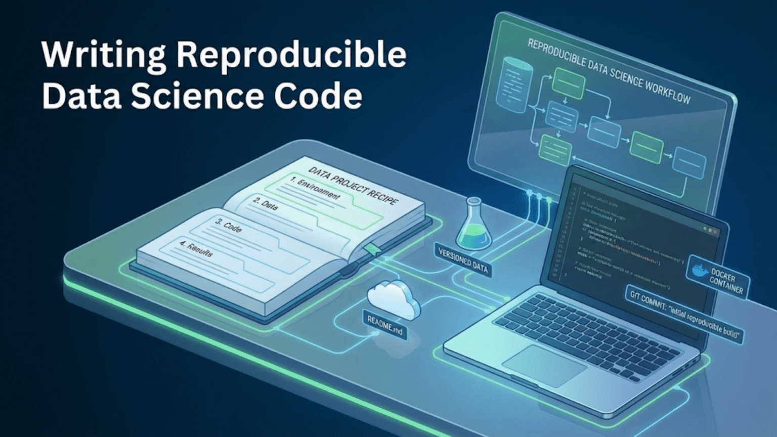
Reproducible data science code is code that produces identical results every time it is run, by anyone, on any compatible machine — now and in the future. Achieving reproducibility requires controlling all sources of randomness through fixed seeds, pinning exact software versions in documented environments, separating configuration from code, version-controlling both code and data, and building deterministic pipelines that can be run end-to-end from raw data to final results with a single command.
Introduction
A researcher publishes a landmark machine learning paper claiming their new architecture achieves state-of-the-art performance on a standard benchmark. Other researchers try to reproduce the result. Months of effort later, the best anyone can get is several percentage points below the claimed number. The original authors can’t reproduce it either — their original training run is gone, the exact environment is unrecoverable, and the random seeds were never recorded.
This scenario, known as the reproducibility crisis, is widespread across data science and machine learning. A 2021 analysis found that the majority of published machine learning results could not be fully reproduced. In industry, the problem is equally costly: models that “worked in the notebook” mysteriously underperform in production, experiments from three months ago can’t be replicated for an audit, and teams spend weeks re-deriving results that should have been a matter of clicking “run.”
Reproducibility is not a luxury or an academic concern — it is a fundamental property of trustworthy, professional data science work. It enables you to verify your own results, share work with confidence, audit models in production, build on previous experiments without starting from scratch, and hand off projects to teammates without the dreaded “it only works on my machine” caveat.
This guide covers every dimension of reproducibility in data science: the sources of non-reproducibility you need to control, the tools and patterns that achieve control, and how to build workflows where reproducibility is the default rather than an afterthought.
Why Data Science Code Is Non-Reproducible by Default
Before learning to achieve reproducibility, understand the forces working against it. Data science code is non-reproducible by default for several interconnected reasons.
Source 1: Uncontrolled Randomness
Machine learning algorithms make random choices at numerous points: weight initialization in neural networks, data shuffling before training, bootstrap sampling in random forests, random feature subsets at each tree split, train/test splitting, dropout during training, k-fold cross-validation splits. If these random choices aren’t fixed, every run produces a different result.
# Non-reproducible: Different split every run
X_train, X_test, y_train, y_test = train_test_split(X, y, test_size=0.2)

# Reproducible: Same split every run
X_train, X_test, y_train, y_test = train_test_split(X, y, test_size=0.2, random_state=42)Source 2: Evolving Software Dependencies
Python packages release new versions constantly. A change in pandas’ groupby behavior between 1.5 and 2.0, a bug fix in scikit-learn’s feature importance calculation, or a numerical precision change in numpy can alter results — even when your code is identical.
# Code that behaved differently across pandas versions
# pandas < 2.0: Silently filled missing with 0
# pandas >= 2.0: Raises FutureWarning and behaves differently
df.fillna(method='ffill')Without pinned dependencies, the same code run six months later may produce different results.
Source 3: Hidden Notebook State
Jupyter Notebooks accumulate hidden state through out-of-order cell execution. A variable defined in one session persists to the next. A cell run twice modifies state cumulatively. The notebook appears to work but only because it depends on the specific execution history of the current session — a history that can never be exactly recreated.
Source 4: Floating-Point Non-Determinism
Floating-point arithmetic can produce different results depending on CPU architecture, thread execution order, and hardware-specific optimizations. Parallel computations on GPU are especially susceptible — the order in which threads complete varies, and floating-point addition is not associative at machine precision.
Source 5: Data Drift and Undocumented Data Sources
If your code reads from a live database or file path that changes over time, running the same code later produces different results because the input data has changed. Without versioning the specific data snapshot used for each experiment, results become impossible to reproduce.
Source 6: Undocumented Manual Steps
“I adjusted the learning rate by hand after epoch 5.” “I removed three outliers that I noticed looked wrong.” “I ran the feature engineering twice because the first run seemed off.” These undocumented manual interventions are invisible in the code but materially affect results.
Pillar 1: Controlling Randomness with Seeds
The most accessible reproducibility improvement is setting random seeds everywhere randomness is used.
Setting Seeds Comprehensively
Different libraries have different random number generators, each of which must be seeded independently:
import random
import numpy as np
import os

def set_all_seeds(seed: int = 42) -> None:
    """
    Set all random seeds for reproducible results.

    Call this function at the very beginning of every script and
    notebook before any data loading or processing.

    Parameters
    ----------
    seed : int, optional
        The random seed value. 42 is conventional. By default 42.
    """
    # Python's built-in random module
    random.seed(seed)

    # NumPy
    np.random.seed(seed)

    # Python hash seed — affects dict ordering and set operations
    os.environ['PYTHONHASHSEED'] = str(seed)

    # TensorFlow (if used)
    try:
        import tensorflow as tf
        tf.random.set_seed(seed)
    except ImportError:
        pass

    # PyTorch (if used)
    try:
        import torch
        torch.manual_seed(seed)
        torch.cuda.manual_seed(seed)
        torch.cuda.manual_seed_all(seed)
        # For full determinism on CUDA (may reduce performance)
        torch.backends.cudnn.deterministic = True
        torch.backends.cudnn.benchmark = False
    except ImportError:
        pass

# Call once at the start of every script/notebook
set_all_seeds(seed=42)The random_state Parameter Convention
Scikit-learn uses a consistent random_state parameter across all algorithms that involve randomness:
from sklearn.model_selection import train_test_split, KFold, cross_val_score
from sklearn.ensemble import RandomForestClassifier, GradientBoostingClassifier
from sklearn.linear_model import LogisticRegression

RANDOM_STATE = 42  # Define once, use everywhere

# Data splitting
X_train, X_test, y_train, y_test = train_test_split(
    X, y,
    test_size=0.2,
    stratify=y,              # Maintain class distribution
    random_state=RANDOM_STATE
)

# Cross-validation
cv = KFold(n_splits=5, shuffle=True, random_state=RANDOM_STATE)

# Models
rf = RandomForestClassifier(
    n_estimators=300,
    max_features='sqrt',
    random_state=RANDOM_STATE
)

gb = GradientBoostingClassifier(
    n_estimators=200,
    learning_rate=0.05,
    random_state=RANDOM_STATE
)

lr = LogisticRegression(
    max_iter=1000,
    random_state=RANDOM_STATE
)

# Hyperparameter search
from sklearn.model_selection import RandomizedSearchCV
search = RandomizedSearchCV(
    rf,
    param_distributions={...},
    n_iter=50,
    random_state=RANDOM_STATE  # Controls which hyperparameter combinations are tried
)Centralizing the seed value in a single constant (RANDOM_STATE = 42) means you can change it in one place and all models/splits update consistently — useful for sensitivity analyses that check whether your conclusions are seed-dependent.
Documenting Seed Choices
# configs/config.yaml
reproducibility:
  random_seed: 42
  # WHY 42: conventional choice; verified on 2024-09-15 that results are
  # stable (±0.002 AUC-ROC) across seeds 1, 7, 42, 123, 2024
# See notebooks/exploratory/08_seed_sensitivity.ipynbPillar 2: Environment Reproducibility
Identical code plus identical data plus different software versions can still produce different results. Environment reproducibility means capturing the exact software stack that produced a given result.
The requirements.txt Hierarchy
For maximum reproducibility, maintain two requirements files:
# requirements.txt — exact pinned versions for full reproducibility
# Generated by: pip freeze > requirements.txt
# Last updated: 2024-09-15

certifi==2023.7.22
joblib==1.3.2
matplotlib==3.7.2
numpy==1.25.2
pandas==2.0.3
scikit-learn==1.3.0
scipy==1.11.2
seaborn==0.12.2
xgboost==1.7.6
# requirements-base.txt — minimum version constraints for flexibility
# Used when installing in environments where exact versions create conflicts
numpy>=1.24,<2.0
pandas>=2.0,<3.0
scikit-learn>=1.3,<2.0
matplotlib>=3.7
seaborn>=0.12
xgboost>=1.7The pinned requirements.txt guarantees exact reproduction on any machine. The flexible requirements-base.txt allows installation in environments with other constraints (Docker base images, shared clusters).
conda environment.yml for Full Stack Reproducibility
For projects using conda (especially those with GPU dependencies or compiled scientific libraries), environment.yml captures the complete environment including Python version and conda packages:
# environment.yml
name: churn-model-v2
channels:
  - conda-forge
  - defaults
dependencies:
  - python=3.11.4
  - pip=23.2.1
  - numpy=1.25.2
  - pandas=2.0.3
  - scikit-learn=1.3.0
  - matplotlib=3.7.2
  - seaborn=0.12.2
  - scipy=1.11.2
  - jupyterlab=4.0.5
  - pip:
    - xgboost==1.7.6
    - shap==0.42.1
    - mlflow==2.6.0
- pandera==0.17.0Docker for Hermetic Environment Reproducibility
For the strongest environment reproducibility guarantee — ensuring not just Python packages but the entire system environment (OS version, system libraries, CUDA version) is controlled — use Docker:
# Dockerfile

# Pin the exact base image with SHA digest for maximum reproducibility
FROM python:3.11.4-slim-bullseye

# Install system dependencies at pinned versions
RUN apt-get update && apt-get install -y \
    libgomp1=12.2.0-14 \
    && rm -rf /var/lib/apt/lists/*

WORKDIR /app

# Copy and install Python dependencies first (Docker layer caching)
COPY requirements.txt .
RUN pip install --no-cache-dir -r requirements.txt

# Copy application code
COPY . .

# Set Python hash seed for reproducibility
ENV PYTHONHASHSEED=42

CMD ["python", "src/train_model.py", "--config", "configs/config.yaml"]With this Dockerfile pinning the base image, system libraries, and Python packages, the exact computational environment is preserved and reproducible years into the future.
Documenting the Environment at Result Time
When publishing a model result or sharing an analysis, record the exact environment state:
import platform
import sys
import pkg_resources

def print_environment_info():
    """Print complete environment information for reproducibility documentation."""
    print(f"Python version: {sys.version}")
    print(f"Platform: {platform.platform()}")
    print(f"Architecture: {platform.machine()}")
    print()

    key_packages = ['numpy', 'pandas', 'scikit-learn', 'xgboost',
                    'matplotlib', 'scipy', 'tensorflow', 'torch']

    print("Key package versions:")
    for pkg in key_packages:
        try:
            version = pkg_resources.get_distribution(pkg).version
            print(f"  {pkg}: {version}")
        except pkg_resources.DistributionNotFound:
            print(f"  {pkg}: not installed")

print_environment_info()Python version: 3.11.4 (main, Jul 5 2023, 13:45:01) [GCC 11.2.0]
Platform: Linux-5.15.0-1040-aws-x86_64-with-glibc2.31
Architecture: x86_64
Key package versions:
numpy: 1.25.2
pandas: 2.0.3
scikit-learn: 1.3.0
xgboost: 1.7.6
matplotlib: 3.7.2
scipy: 1.11.2Include this output in your notebook results or model documentation.
Pillar 3: Separating Configuration from Code
Hardcoded values — file paths, column names, hyperparameters, thresholds — are one of the most common reproducibility killers. When they’re embedded in code, changing an experiment requires modifying source files, which creates ambiguity about what changed between runs.
The Configuration File Approach
Centralize all experiment parameters in version-controlled YAML or JSON files:
# configs/config.yaml

experiment:
  name: "xgboost_v3_tuned"
  description: "XGBoost with learning rate decay and L1 regularization"
  date: "2024-09-15"
  author: "Jane Smith"

reproducibility:
  random_seed: 42

paths:
  raw_data: "data/raw/transactions_2024_q3.csv"
  processed_data: "data/processed/features_v2.parquet"
  model_output: "models/xgboost_v3.pkl"
  metrics_output: "reports/metrics/xgboost_v3_metrics.json"
  figures_dir: "reports/figures/"

data:
  target_column: "churned"
  id_column: "customer_id"
  date_column: "transaction_date"
  categorical_columns: ["channel", "product_category", "region"]
  numerical_columns: ["amount", "frequency_90d", "recency_days"]
  test_size: 0.2
  validation_size: 0.1

model:
  algorithm: "xgboost"
  hyperparameters:
    n_estimators: 500
    learning_rate: 0.05
    max_depth: 6
    min_child_weight: 3
    subsample: 0.8
    colsample_bytree: 0.8
    gamma: 0.1
    reg_alpha: 0.2
    reg_lambda: 1.5
    scale_pos_weight: 3.2

evaluation:
  primary_metric: "roc_auc"
  threshold: 0.42
metrics: ["roc_auc", "f1", "precision", "recall", "average_precision"]Load and use consistently:
import yaml
from pathlib import Path
from typing import Any

def load_config(config_path: str = "configs/config.yaml") -> dict[str, Any]:
    """Load configuration from YAML file."""
    with open(config_path, 'r') as f:
        config = yaml.safe_load(f)
    return config


def train(config_path: str = "configs/config.yaml") -> None:
    config = load_config(config_path)

    seed = config['reproducibility']['random_seed']
    set_all_seeds(seed)

    # All paths from config — never hardcoded
    data_path = config['paths']['processed_data']
    model_path = config['paths']['model_output']

    # All hyperparameters from config
    hyperparams = config['model']['hyperparameters']
    model = XGBClassifier(**hyperparams, random_state=seed)

    # ...


if __name__ == "__main__":
    import argparse
    parser = argparse.ArgumentParser()
    parser.add_argument("--config", default="configs/config.yaml")
    args = parser.parse_args()
train(config_path=args.config)Now different experiments use different config files — and the exact config used for each result is recorded alongside the results.
Versioning Config Files with Experiments
Create a config file for each significant experiment variant:
configs/
├── config.yaml             ← Current/default config
├── experiments/
│   ├── exp_01_baseline.yaml
│   ├── exp_02_feature_engineering_v2.yaml
│   ├── exp_03_xgboost_default.yaml
│   ├── exp_04_xgboost_tuned.yaml
│ └── exp_05_xgboost_v2_more_regularization.yamlThe config file becomes the identity of the experiment — commit each new config to Git and the complete experiment is reproducible forever.
Pillar 4: Data Version Control
Code versioning with Git is well understood. Data versioning is equally important but much less commonly practiced.
The Problem
Code version: commit a3f8c2d  (Git commit — easy to track)
Data version: transactions_2024_q3.csv (??? — which version? updated monthly!)When a colleague reports a discrepancy in your model’s performance, you need to know not just what code was used, but what data. Without data versioning, this question is unanswerable.
DVC: Data Version Control
DVC extends Git semantics to data and model files. DVC tracks data files by their content hash, stores them in remote storage (S3, GCS, Azure Blob), and records the mapping between Git commits and data versions.
# Set up DVC
pip install dvc dvc-s3
dvc init

# Configure remote storage
dvc remote add -d myremote s3://my-bucket/dvc-store

# Track a data file
dvc add data/raw/transactions_2024_q3.csv
# Creates: data/raw/transactions_2024_q3.csv.dvc (text file, committed to Git)
# The CSV itself: goes into .dvc/cache and pushed to S3

# Commit the .dvc file to Git
git add data/raw/transactions_2024_q3.csv.dvc
git commit -m "Add Q3 2024 transaction data"

# Push data to S3
dvc push

# Six months later, anyone can reproduce exactly:
git checkout a3f8c2d        # Check out the code version
dvc pull                    # Pull the exact data version that code used
python src/train_model.py # Identical results guaranteedThe .dvc file is tiny (a few lines of JSON), lives in Git, and records a SHA256 hash of the data file. Checking out a commit and running dvc pull retrieves exactly the data that was used when that commit was made.
Tracking Processed Data and Models
DVC can also track intermediate data and trained models:
# Track processed features
dvc add data/processed/features_v2.parquet

# Track trained model
dvc add models/xgboost_v3.pkl

# Now you have full lineage: raw data → processed → model
# All three are tied to specific Git commits and reproducibleLightweight Alternative: Data Hashing
If DVC is too heavyweight for a project, at minimum record the hash of your data files alongside your results:
import hashlib

def compute_file_hash(filepath: str, algorithm: str = 'sha256') -> str:
    """Compute cryptographic hash of a file for reproducibility documentation."""
    h = hashlib.new(algorithm)
    with open(filepath, 'rb') as f:
        for chunk in iter(lambda: f.read(65536), b''):
            h.update(chunk)
    return h.hexdigest()

# Record with your results
data_hash = compute_file_hash("data/raw/transactions_2024_q3.csv")
print(f"Training data SHA256: {data_hash}")
# Training data SHA256: 3b4f8c2d9e1a6f7b8c3d4e5f6a7b8c9d0e1f2a3b4c5d6e7f8a9b0c1d2e3f4a5bRecord this hash in your experiment log and model documentation. When someone asks “which data version trained this model?”, you can verify by comparing hashes.
Pillar 5: Building End-to-End Reproducible Pipelines
Reproducibility isn’t just about individual scripts — it’s about the entire pipeline from raw data to final results being executable deterministically.
The End-to-End Pipeline Pattern
Every data science project should have a single command that runs the complete pipeline:
# src/pipeline.py

import argparse
import logging
from pathlib import Path

from src.data.make_dataset import download_raw_data
from src.data.preprocess import preprocess_transactions
from src.features.build_features import build_feature_matrix
from src.models.train_model import train_model
from src.models.evaluate_model import evaluate_model
from src.utils.config import load_config
from src.utils.reproducibility import set_all_seeds, log_environment

logging.basicConfig(level=logging.INFO)
logger = logging.getLogger(__name__)


def run_pipeline(config_path: str) -> dict:
    """
    Run the complete ML pipeline end-to-end.

    Parameters
    ----------
    config_path : str
        Path to the experiment configuration YAML file.

    Returns
    -------
    dict
        Dictionary of evaluation metrics from the trained model.
    """
    # Load configuration
    config = load_config(config_path)
    logger.info(f"Running pipeline: {config['experiment']['name']}")

    # Set reproducibility
    seed = config['reproducibility']['random_seed']
    set_all_seeds(seed)
    logger.info(f"Random seed set to {seed}")

    # Log environment for documentation
    log_environment()

    # Step 1: Data ingestion
    logger.info("Step 1: Data ingestion")
    raw_data = download_raw_data(config['paths']['raw_data'])

    # Step 2: Preprocessing
    logger.info("Step 2: Preprocessing")
    clean_data = preprocess_transactions(raw_data, config)
    clean_data.to_parquet(
        config['paths']['interim_data'],
        index=False
    )

    # Step 3: Feature engineering
    logger.info("Step 3: Feature engineering")
    features = build_feature_matrix(clean_data, config)
    features.to_parquet(
        config['paths']['processed_data'],
        index=False
    )

    # Step 4: Model training
    logger.info("Step 4: Model training")
    model, metrics = train_model(features, config)

    # Step 5: Evaluation
    logger.info("Step 5: Evaluation")
    final_metrics = evaluate_model(model, features, config)

    # Save results
    import json
    metrics_path = config['paths']['metrics_output']
    Path(metrics_path).parent.mkdir(parents=True, exist_ok=True)

    results = {
        'experiment_name': config['experiment']['name'],
        'config_path': config_path,
        'random_seed': seed,
        'metrics': final_metrics
    }

    with open(metrics_path, 'w') as f:
        json.dump(results, f, indent=2)

    logger.info(f"Pipeline complete. Metrics: {final_metrics}")
    return final_metrics


if __name__ == "__main__":
    parser = argparse.ArgumentParser(description="Run the ML pipeline")
    parser.add_argument(
        "--config",
        type=str,
        default="configs/config.yaml",
        help="Path to configuration file"
    )
    args = parser.parse_args()
run_pipeline(args.config)Run any experiment:
# Run with default config
python src/pipeline.py

# Run a specific experiment
python src/pipeline.py --config configs/experiments/exp_04_xgboost_tuned.yaml

# Reproduce a historical experiment from Git history
git checkout a3f8c2d
python src/pipeline.py --config configs/experiments/exp_03_xgboost_default.yamlMakefile Automation
Expose pipeline commands through a Makefile for discoverability:
# Makefile

PYTHON = python
CONFIG = configs/config.yaml

.PHONY: all data features train evaluate test clean reproduce

all: data features train evaluate

data:
	$(PYTHON) src/data/make_dataset.py --config $(CONFIG)

features:
	$(PYTHON) src/features/build_features.py --config $(CONFIG)

train:
	$(PYTHON) src/models/train_model.py --config $(CONFIG)

evaluate:
	$(PYTHON) src/models/evaluate_model.py --config $(CONFIG)

# Run complete pipeline
pipeline:
	$(PYTHON) src/pipeline.py --config $(CONFIG)

# Reproduce a specific experiment
reproduce:
	@echo "Reproducing experiment: $(EXPERIMENT)"
	$(PYTHON) src/pipeline.py --config configs/experiments/$(EXPERIMENT).yaml

test:
	pytest tests/ -v --tb=short

# Full reproduction check: git clone fresh, run pipeline, compare metrics
reproduce-check:
	git stash
	dvc pull
	$(PYTHON) src/pipeline.py --config $(CONFIG)
$(PYTHON) scripts/compare_metrics.py --expected reports/expected_metrics.jsonUsage:
make pipeline                                    # Run default pipeline
make reproduce EXPERIMENT=exp_04_xgboost_tuned  # Reproduce specific experiment
make reproduce-check # Verify full reproducibilityPillar 6: Experiment Tracking
Manually managing experiment results in files and spreadsheets is error-prone and doesn’t scale. Dedicated experiment tracking tools record parameters, metrics, artifacts, and environment automatically.
MLflow: The Open-Source Standard
MLflow is the most widely adopted open-source experiment tracking tool. It logs parameters, metrics, artifacts, and model files for each experiment run, and provides a web UI for comparing runs.
import mlflow
import mlflow.sklearn

from src.utils.config import load_config
from src.utils.reproducibility import set_all_seeds

def train_with_tracking(config_path: str) -> None:
    config = load_config(config_path)
    seed = config['reproducibility']['random_seed']
    set_all_seeds(seed)

    # Start an MLflow run
    with mlflow.start_run(run_name=config['experiment']['name']):

        # Log all configuration parameters
        mlflow.log_params({
            'random_seed': seed,
            'algorithm': config['model']['algorithm'],
            **config['model']['hyperparameters']
        })

        # Log data information
        mlflow.log_param('training_data', config['paths']['processed_data'])
        mlflow.log_param('test_size', config['data']['test_size'])

        # ... load data, train model ...

        # Log metrics
        mlflow.log_metrics({
            'roc_auc': metrics['roc_auc'],
            'f1_score': metrics['f1'],
            'precision': metrics['precision'],
            'recall': metrics['recall']
        })

        # Log the trained model
        mlflow.sklearn.log_model(model, "model")

        # Log the config file as an artifact
        mlflow.log_artifact(config_path, "config")

        # Log figures
        mlflow.log_artifact("reports/figures/roc_curve.png", "figures")

        print(f"Run ID: {mlflow.active_run().info.run_id}")
print(f"AUC-ROC: {metrics['roc_auc']:.4f}")Start the MLflow UI:
mlflow ui
# Opens at http://localhost:5000The UI shows all experiments in a table, allows sorting and filtering by metric, and lets you compare the parameters and metrics of any two runs side by side — answering “what changed between the run that got 0.891 and the one that got 0.914?” in seconds.
Reproducing a Specific MLflow Run
import mlflow

# Load a specific run by its ID
run_id = "3f8c2d9e1a6f7b8c3d4e5f6a7b8c9d0e"
run = mlflow.get_run(run_id)

# Get all parameters from that run
params = run.data.params
print(f"Random seed used: {params['random_seed']}")
print(f"Learning rate: {params['learning_rate']}")

# Load the exact model artifact
model = mlflow.sklearn.load_model(f"runs:/{run_id}/model")Weights & Biases and Neptune
For teams with more complex needs — deep learning training curves, hyperparameter sweep visualization, team collaboration — Weights & Biases (W&B) and Neptune offer richer tracking capabilities with hosted infrastructure, though they require API keys and have usage costs beyond free tiers.
import wandb

wandb.init(
    project="customer-churn",
    config=config,
    name=config['experiment']['name']
)

# Log metrics during training
for epoch in range(n_epochs):
    wandb.log({
        'train_loss': train_loss,
        'val_auc': val_auc,
        'epoch': epoch
    })

wandb.finish()Pillar 7: Making Notebooks Reproducible
Notebooks require special attention because their stateful execution model works against reproducibility.
The Notebook Reproducibility Checklist
Before sharing or archiving any notebook:
1. Restart and run all cells
- Kernel → Restart & Run All — if the notebook fails, it is not reproducible
- This is non-negotiable for report notebooks shared with others
2. Clear and re-run, verify determinism
- Run it twice. Do the results match exactly?
- If not, there’s uncontrolled randomness somewhere
3. Set the seed at the very first code cell
# Cell 1 — always the first code cell in every notebook
import random
import numpy as np
import os

SEED = 42
random.seed(SEED)
np.random.seed(SEED)
os.environ['PYTHONHASHSEED'] = str(SEED)4. Use absolute or project-relative paths
from pathlib import Path

# Don't:
df = pd.read_csv("/Users/jane/Desktop/project/data/data.csv")  # Absolute

# Do:
PROJECT_ROOT = Path(__file__).parent.parent  # Or Path("../..") in a notebook
df = pd.read_csv(PROJECT_ROOT / "data" / "raw" / "data.csv")5. Print versions and environment info
# First markdown cell or early code cell
import sys, pandas, numpy, sklearn
print(f"Python: {sys.version}")
print(f"pandas: {pandas.__version__}")
print(f"numpy: {numpy.__version__}")
print(f"scikit-learn: {sklearn.__version__}")Papermill: Parameterized Notebook Execution
Papermill executes notebooks programmatically with injected parameters, enabling notebooks to be part of automated, reproducible pipelines:
# In the notebook: mark a cell as "parameters" tag in Jupyter
# This cell's values can be overridden by Papermill

# parameters
DATA_PATH = "data/processed/features_v2.parquet"
MODEL_CONFIG = "configs/config.yaml"
OUTPUT_PATH = "reports/run_20240915/"
SEED = 42
# Execute the notebook with different parameters
papermill notebooks/reports/model_evaluation.ipynb \
reports/run_20240916/evaluation.ipynb \
-p DATA_PATH "data/processed/features_v3.parquet" \
-p MODEL_CONFIG "configs/experiments/exp_05.yaml" \
-p SEED 42
# The output notebook contains all results with the injected parametersThis transforms notebooks from interactive documents into reproducible, parameterizable pipeline components.
Pillar 8: Testing for Reproducibility
Automated tests can verify reproducibility as part of your CI/CD pipeline — catching accidental non-reproducibility before it reaches production.
Reproducibility Tests
# tests/test_reproducibility.py

import pytest
import numpy as np
import pandas as pd
from sklearn.metrics import roc_auc_score

from src.utils.reproducibility import set_all_seeds
from src.features.build_features import build_feature_matrix
from src.models.train_model import train_model
from src.utils.config import load_config


class TestReproducibility:

    def test_feature_engineering_is_deterministic(self, sample_transactions):
        """Feature engineering must produce identical output across calls."""
        config = load_config("configs/config.yaml")

        set_all_seeds(42)
        features_run1 = build_feature_matrix(sample_transactions, config)

        set_all_seeds(42)
        features_run2 = build_feature_matrix(sample_transactions, config)

        pd.testing.assert_frame_equal(features_run1, features_run2)

    def test_model_training_is_reproducible(self, sample_features):
        """Two training runs with the same seed must produce identical predictions."""
        config = load_config("configs/config.yaml")

        set_all_seeds(42)
        model1, _ = train_model(sample_features, config)
        predictions1 = model1.predict_proba(sample_features.drop('churned', axis=1))[:, 1]

        set_all_seeds(42)
        model2, _ = train_model(sample_features, config)
        predictions2 = model2.predict_proba(sample_features.drop('churned', axis=1))[:, 1]

        np.testing.assert_array_equal(predictions1, predictions2,
            err_msg="Model predictions differ across runs with same seed")

    def test_different_seeds_produce_different_results(self, sample_features):
        """Verify that seed actually affects training (not silently ignored)."""
        config = load_config("configs/config.yaml")

        set_all_seeds(42)
        model1, _ = train_model(sample_features, config)
        preds1 = model1.predict_proba(sample_features.drop('churned', axis=1))[:, 1]

        set_all_seeds(999)
        model2, _ = train_model(sample_features, config)
        preds2 = model2.predict_proba(sample_features.drop('churned', axis=1))[:, 1]

        # Different seeds should produce measurably different models
        assert not np.array_equal(preds1, preds2), \
            "Different seeds produced identical results — seed may not be working"

    def test_pipeline_metrics_match_expected(self):
        """Golden test: full pipeline must reproduce known-good metrics."""
        EXPECTED_AUC = 0.9142  # Recorded from verified run on 2024-09-15
        TOLERANCE = 0.001

        config = load_config("configs/config.yaml")
        metrics = run_pipeline("configs/config.yaml")

        assert abs(metrics['roc_auc'] - EXPECTED_AUC) < TOLERANCE, \
f"AUC-ROC {metrics['roc_auc']:.4f} differs from expected {EXPECTED_AUC:.4f}"The last test — a golden test — is particularly powerful: it records the exact metric achieved on a specific date with a specific environment, and fails the build if future changes cause any unexplained deviation. This catches dependency upgrades, code refactors, and other changes that silently affect model performance.
Reproducibility Documentation: The Experiment Report
Every significant experiment should be accompanied by a structured report that contains everything needed to reproduce it:
# Experiment Report: XGBoost v3 — Tuned Hyperparameters

## Experiment Summary
- **Date**: 2024-09-15
- **Author**: Jane Smith
- **Goal**: Improve AUC-ROC over XGBoost v2 baseline (0.908) using
  Bayesian hyperparameter optimization

## How to Reproduce

    git checkout a3f8c2d
    dvc pull
    python src/pipeline.py --config configs/experiments/exp_04_xgboost_tuned.yaml

Expected result: AUC-ROC = 0.9142 ± 0.0005

## Environment
- Python: 3.11.4
- Key packages: numpy==1.25.2, pandas==2.0.3, scikit-learn==1.3.0,
  xgboost==1.7.6
- Platform: Linux x86_64 (AWS t3.xlarge)

## Data
- Training: data/raw/transactions_2024_q1_q2.csv
  (SHA256: 3b4f8c2d9e1a6f7b8c3d4e5f6a7b8c9d...)
- Test: data/raw/transactions_2024_q3.csv
  (SHA256: 7f2a1b9c4e5d6a3b8c2d1e4f5a6b7c8d...)

## Configuration
Full config: configs/experiments/exp_04_xgboost_tuned.yaml
Random seed: 42 (stable across seeds 1, 7, 42, 123 — sensitivity verified)

## Results

| Metric | Value |
|--------|-------|
| AUC-ROC | 0.9142 |
| F1 Score | 0.847 |
| Precision | 0.856 |
| Recall | 0.839 |

## What Changed from v2
- Reduced learning_rate from 0.1 to 0.05 (slower learning, better generalization)
- Added L1 regularization (reg_alpha=0.2)
- Increased n_estimators from 300 to 500 (more trees to compensate for lower lr)

## MLflow Run
- Run ID: 3f8c2d9e1a6f7b8c3d4e5f6a7b8c9d0e
- Experiment: customer-churn-model
Common Reproducibility Pitfalls and Their Fixes
| Pitfall | Symptom | Fix |
|---|---|---|
| Missing random seed | Results differ between runs | Set seed in set_all_seeds() at script start |
| Unpinned dependencies | Results differ after pip install --upgrade | Use pip freeze > requirements.txt |
| Fitting on test data | Optimistic validation metrics | Fit all preprocessors only on training data |
| Absolute file paths | Code fails on other machines | Use relative paths + pathlib.Path |
| Manual steps not in code | “It only works when I run it manually” | Automate all steps in pipeline scripts |
| Data changes over time | Can’t reproduce old results | Version data with DVC; record data hashes |
| Notebook hidden state | Results depend on execution order | Restart & Run All before sharing |
| No experiment records | “What params produced that result?” | Use MLflow or structured experiment log |
| PyTorch non-determinism | GPU results differ each run | Set torch.backends.cudnn.deterministic = True |
| Parallel processing order | Results differ with multiprocessing | Use deterministic algorithms; sort before parallel ops |
Summary
Reproducibility is not a single technique but a discipline — a set of interconnected practices that together guarantee your results can be trusted, verified, and recreated. The eight pillars covered in this guide — controlling randomness through seeds, pinning environments, separating configuration from code, versioning data with DVC, building end-to-end pipelines, tracking experiments with MLflow, making notebooks reproducible, and testing for reproducibility — address the full range of sources through which non-reproducibility creeps into data science work.
The payoff for this investment is substantial and compounds over time. Reproducible projects can be audited, extended, and handed off without loss of knowledge. Reproducible experiments enable genuine scientific comparison of approaches. Reproducible models can be debugged in production when they fail. And reproducible workflows build the professional trust that distinguishes mature data science practice from ad-hoc analysis.
The practical path forward is incremental: start with seeds and pinned dependencies (the highest-impact, lowest-effort changes), then add config files and a pipeline script, then DVC for data, then MLflow for experiment tracking. Each step builds on the previous, and the cumulative effect is a fully reproducible, professionally credible data science practice.
Key Takeaways
- Reproducibility has eight interconnected sources of failure — randomness, software versions, notebook state, floating-point precision, data drift, and undocumented manual steps — and each must be addressed for full reproducibility
set_all_seeds()must seed Python’srandommodule, NumPy, PyTorch, TensorFlow, andPYTHONHASHSEED— seeding only one or two is insufficient for full determinismpip freeze > requirements.txtcaptures the exact software environment;environment.ymldoes the same for conda — always pin exact versions for reproducible experiments- Config YAML files separate all experiment parameters from code — enabling different experiments to run by swapping config files, with Git tracking what changed between them
- DVC extends Git semantics to data files, enabling
git checkout + dvc pullto retrieve the exact code and data used for any historical result - MLflow (or equivalent) automatically records parameters, metrics, artifacts, and environment for every training run, answering “what parameters produced that result?” without manual documentation
Kernel → Restart & Run Allbefore sharing any notebook is non-negotiable — it’s the only way to verify a notebook is actually reproducible rather than depending on hidden session state- Golden tests — automated tests that verify the pipeline produces metrics matching a known-good result from a verified run — catch reproducibility regressions before they reach production