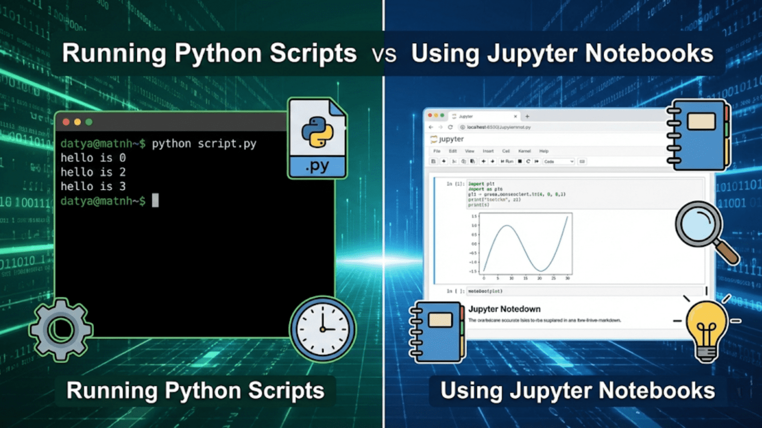
Python scripts (.py files) and Jupyter Notebooks (.ipynb files) are two primary ways to write and execute Python code, each suited for different tasks. Python scripts run sequentially from top to bottom and are ideal for production code and automation, while Jupyter Notebooks allow you to run code in interactive cells, making them perfect for data exploration, visualization, and storytelling with data.
Introduction
If you’ve ever worked with Python in a data science context, you’ve probably come across two very different environments: the classic Python script — a plain .py file run from the terminal — and the Jupyter Notebook — an interactive, browser-based document where code, text, and visuals live side by side.
Both tools use Python. Both can do extraordinary things. But they are built for fundamentally different workflows, and choosing the wrong one for the job can slow you down, introduce bugs, or make collaboration harder than it needs to be.
This article is your complete guide to understanding Python scripts and Jupyter Notebooks: what they are, how they work, when to use each, and how professional data scientists combine them in real projects. Whether you’re a beginner trying to figure out where to type your first line of code, or an intermediate practitioner looking to tighten up your workflow, this guide will give you the clarity and confidence to make the right choice every single time.
What Is a Python Script?
A Python script is a plain text file with a .py extension that contains Python code written to be executed from start to finish. You write your code in any text editor or IDE (like VS Code, PyCharm, or even Notepad), save the file, and then run it from the command line or terminal using the command:
python my_script.pyPython reads the file from the top and executes every line in order. When it reaches the end of the file, it stops. There’s no interactivity during execution — unless you’ve specifically coded for user input — and the output is printed to the terminal or saved to a file.
A Simple Python Script Example
Here’s what a simple Python script might look like:
# data_analysis.py

import pandas as pd

# Load the data
df = pd.read_csv("sales_data.csv")

# Compute summary statistics
summary = df.describe()

# Print results
print(summary)

# Save to file
summary.to_csv("summary_output.csv")You save this as data_analysis.py, run python data_analysis.py in your terminal, and it executes every line from top to bottom. If there’s an error on line 7, the script crashes and nothing after that line runs.
Key Characteristics of Python Scripts
- Sequential execution: Code runs from line 1 to the last line in order
- Non-interactive: The user doesn’t interact mid-execution (unless coded to do so)
- File format: Plain
.pytext files that any text editor can open - Reproducibility: Running the script again produces the same result (assuming input data hasn’t changed)
- Automation-friendly: Scripts can be scheduled using cron jobs or task schedulers
- Version control:
.pyfiles work seamlessly with Git and other version control systems
What Is a Jupyter Notebook?
A Jupyter Notebook is an interactive, web-based computing environment that lets you write and execute Python code in small, individual blocks called cells. Each cell can contain code, formatted text (Markdown), equations (LaTeX), or visualizations — all in one document.
When you run a cell, only that cell’s code executes, and its output appears directly below it. You can run cells in any order, re-run them with changes, and see results immediately without re-running your entire program.
Jupyter Notebooks are saved as .ipynb files, which are actually JSON documents storing your code, outputs, and metadata together.
Launching Jupyter
You launch Jupyter from your terminal:
jupyter notebookThis opens a browser window showing your file system. You create a new notebook, and you’re presented with an empty interface where you can start adding cells.
A Simple Jupyter Notebook Cell Example
In a Jupyter Notebook, you might have separate cells like:
Cell 1:
import pandas as pd
df = pd.read_csv("sales_data.csv")
df.head()Output: A nicely formatted table showing the first 5 rows
Cell 2:
df.describe()Output: Summary statistics table
Cell 3:
import matplotlib.pyplot as plt
df['revenue'].plot(kind='bar')
plt.title("Revenue by Region")
plt.show()Output: A bar chart displayed directly in the notebook
Each cell runs independently. You can edit Cell 2, re-run only that cell, and see updated results without re-running your data loading code in Cell 1. This is the core power of Jupyter.
Key Characteristics of Jupyter Notebooks
- Cell-by-cell execution: Run individual blocks of code independently
- Interactive output: See results, plots, and tables inline immediately
- Mixed content: Combine code, explanatory text, and visuals in one document
- Exploratory: Ideal for trying things out and iterating quickly
- Shareable: Notebooks can be exported as HTML, PDF, or shared via platforms like GitHub, Google Colab, or NBViewer
- Non-linear execution risk: Cells can be run out of order, which can introduce hidden state bugs
Core Differences: Python Scripts vs Jupyter Notebooks
Understanding the fundamental differences between these two tools helps you choose the right one for any given situation.
| Feature | Python Script (.py) | Jupyter Notebook (.ipynb) |
|---|---|---|
| Execution model | Top to bottom, all at once | Cell by cell, in any order |
| Interactivity | Non-interactive (by default) | Highly interactive |
| Output display | Terminal / log files | Inline (below each cell) |
| Visualization | Requires saving to file or pop-up window | Renders directly in the document |
| File size | Small, plain text | Larger (stores outputs in JSON) |
| Version control | Excellent (clean diffs with Git) | Challenging (outputs inflate diffs) |
| Automation | Easy to schedule and automate | Not designed for direct automation |
| Collaboration | Best with IDEs and Git | Best for sharing results and analysis |
| Best use case | Production code, pipelines, apps | Exploration, EDA, teaching, reporting |
| State management | Stateless after each run | Maintains state across cell executions |
| Reproducibility | Highly reproducible | Risk of hidden state from out-of-order execution |
| Startup time | Instant (just run the file) | Requires browser, kernel startup |
Understanding Execution Models in Depth
One of the most important — and most misunderstood — differences between scripts and notebooks is how they handle state and execution order.
Script Execution: Linear and Predictable
When Python runs a script, it creates a fresh Python interpreter, executes every line from top to bottom, and then destroys the interpreter. If you run the script again, everything starts fresh. There’s no memory of previous runs.
This makes scripts predictable and reliable. If you share your script with someone and they run it on the same data, they’ll get the exact same result. Every single time.
Notebook Execution: Flexible but Stateful
Jupyter Notebooks maintain a kernel — a running Python process — that persists as long as the notebook is open. Every cell you run modifies the kernel’s state. Variables you define in one cell are available in all subsequent cells.
The problem is that cells can be run in any order. Here’s a classic example of the danger this creates:
Cell 1:
x = 10Cell 2:
x = x * 2
print(x) # Output: 20Cell 3:
x = 100If you run Cell 1, then Cell 2, you get 20. But if you then run Cell 2 again, you get 40. If you run Cell 3 and then Cell 2, you get 200. The output of Cell 2 depends entirely on what order you’ve run other cells — something that isn’t obvious just by reading the notebook.
This “hidden state” problem is one of the most common sources of bugs and confusion in Jupyter Notebooks, especially for beginners. The solution is to periodically use Kernel > Restart & Run All to verify your notebook runs correctly from top to bottom.
When to Use Jupyter Notebooks
Jupyter Notebooks shine in specific scenarios. Here’s a detailed breakdown of when notebooks are the right tool.
1. Exploratory Data Analysis (EDA)
EDA is the process of loading a dataset and examining it from many angles to understand its structure, distributions, relationships, and anomalies. This process is inherently interactive — you look at a histogram, notice something interesting, pivot to look at a correlation matrix, discover a weird value, drill down further.
Notebooks are perfect for EDA because:
- You can run one cell at a time as your thinking evolves
- Plots and tables appear inline, letting you see results without switching windows
- You can annotate your findings in Markdown cells as you go
- You can easily go back and re-run earlier cells with tweaked parameters
# EDA workflow in a Jupyter Notebook

# Cell 1: Load and inspect
import pandas as pd
df = pd.read_csv("customer_data.csv")
print(df.shape)
df.head()

# Cell 2: Check missing values
df.isnull().sum()

# Cell 3: Distribution of age
import matplotlib.pyplot as plt
df['age'].hist(bins=20)
plt.xlabel("Age")
plt.title("Age Distribution")
plt.show()

# Cell 4: Correlation heatmap
import seaborn as sns
sns.heatmap(df.corr(), annot=True, cmap='coolwarm')
plt.show()Each cell here builds on knowledge from the previous one, and you can jump around as your curiosity guides you.
2. Prototyping Machine Learning Models
When building a machine learning model for the first time, you’re constantly experimenting — trying different algorithms, adjusting hyperparameters, comparing results. Notebooks let you do this iteratively without re-running expensive data loading and preprocessing steps every time.
# Cell 1: Load and preprocess (run once)
from sklearn.model_selection import train_test_split
from sklearn.preprocessing import StandardScaler

X = df.drop('target', axis=1)
y = df['target']

X_train, X_test, y_train, y_test = train_test_split(X, y, test_size=0.2, random_state=42)

scaler = StandardScaler()
X_train_scaled = scaler.fit_transform(X_train)
X_test_scaled = scaler.transform(X_test)

# Cell 2: Try Logistic Regression (can re-run independently)
from sklearn.linear_model import LogisticRegression
from sklearn.metrics import accuracy_score

lr = LogisticRegression()
lr.fit(X_train_scaled, y_train)
print(f"LR Accuracy: {accuracy_score(y_test, lr.predict(X_test_scaled)):.4f}")

# Cell 3: Try Random Forest (without re-running Cell 1)
from sklearn.ensemble import RandomForestClassifier

rf = RandomForestClassifier(n_estimators=100, random_state=42)
rf.fit(X_train, y_train)
print(f"RF Accuracy: {accuracy_score(y_test, rf.predict(X_test)):.4f}")You run Cell 1 once to prepare your data, then freely experiment with different models in subsequent cells.
3. Teaching and Presentations
Jupyter Notebooks are widely used in education and data science communication because they combine narrative text with live, executable code. A teacher can write:
- A Markdown cell explaining the concept of gradient descent
- A code cell showing the algorithm in action
- A visualization cell plotting how the loss decreases over epochs
- Another Markdown cell with exercises for students
This narrative + code combination makes notebooks ideal for tutorials, course materials, research papers (through tools like JupyterBook), and conference presentations.
4. Creating Data Reports and Dashboards
Notebooks can be converted to HTML, PDF, or slides, making them useful for generating reports that include live code and outputs. Tools like Papermill let you parameterize notebooks and run them automatically to generate updated reports when new data arrives.
5. Sharing and Collaboration on Analysis
When you want to share an analysis with a colleague or stakeholder who isn’t deeply technical, a notebook is ideal. They can see your code, your reasoning (in text cells), and your outputs all in one place. GitHub renders .ipynb files automatically, making them easy to review without running them.
When to Use Python Scripts
Python scripts are the professional standard for code that needs to be deployed, automated, or maintained over time. Here are the key scenarios where scripts are the better choice.
1. Production Code and Deployment
When you’ve finished exploring and you’re ready to deploy a model or data pipeline, you need to put your code in a .py script. Web applications, APIs, data pipelines, and scheduled jobs all rely on Python scripts, not notebooks.
For example, a Flask API to serve a machine learning model:
# app.py
from flask import Flask, request, jsonify
import pickle
import numpy as np

app = Flask(__name__)

# Load the trained model
with open('model.pkl', 'rb') as f:
    model = pickle.load(f)

@app.route('/predict', methods=['POST'])
def predict():
    data = request.json['features']
    features = np.array(data).reshape(1, -1)
    prediction = model.predict(features)[0]
    return jsonify({'prediction': int(prediction)})

if __name__ == '__main__':
app.run(debug=True)This code is designed to run continuously as a server — something a Jupyter Notebook can’t do.
2. Automated Data Pipelines
If you need to run data processing every night at midnight, every hour, or whenever a new file lands in a folder, you need a Python script. Notebooks don’t integrate well with schedulers like cron (Linux/Mac) or Windows Task Scheduler.
# etl_pipeline.py
import pandas as pd
from datetime import datetime
import logging

logging.basicConfig(filename='pipeline.log', level=logging.INFO)

def extract():
    df = pd.read_csv("raw_data.csv")
    logging.info(f"Extracted {len(df)} rows at {datetime.now()}")
    return df

def transform(df):
    df = df.dropna()
    df['date'] = pd.to_datetime(df['date'])
    df['revenue'] = df['revenue'].astype(float)
    return df

def load(df):
    df.to_csv("processed_data.csv", index=False)
    logging.info(f"Loaded {len(df)} rows to processed_data.csv")

if __name__ == '__main__':
    raw = extract()
    clean = transform(raw)
load(clean)This script can be scheduled to run automatically, log its activity, and process data without any human involvement.
3. Building Reusable Modules and Packages
Python’s module system is built around .py files. When you want to create a utility function that’s used across multiple projects, you write it in a script and import it:
# utils.py
def clean_text(text):
    """Remove whitespace and convert to lowercase."""
    return text.strip().lower()

def calculate_rmse(actual, predicted):
    """Calculate Root Mean Squared Error."""
    import numpy as np
return np.sqrt(np.mean((actual - predicted) ** 2))Then in another script:
from utils import clean_text, calculate_rmseYou can’t do this cleanly with notebook cells.
4. Command-Line Tools
Scripts can accept command-line arguments using the argparse library, making them flexible tools that can be configured at run time:
# train_model.py
import argparse

def main():
    parser = argparse.ArgumentParser(description='Train a classification model')
    parser.add_argument('--data', type=str, required=True, help='Path to training data')
    parser.add_argument('--model', type=str, default='random_forest', help='Model type')
    parser.add_argument('--output', type=str, default='model.pkl', help='Output path')

    args = parser.parse_args()

    print(f"Training {args.model} on {args.data}...")
    # Training logic here...
    print(f"Model saved to {args.output}")

if __name__ == '__main__':
main()Run it as:
python train_model.py --data customer_data.csv --model logistic --output lr_model.pkl5. Large-Scale Data Processing
For processing large datasets that take minutes or hours to run, scripts are more efficient. They have lower memory overhead than notebooks (no browser, no kernel management overhead), can be monitored through logging, and can be run in the background without occupying your interactive session.
6. Testing and Code Quality
Software engineering best practices — unit testing, linting, type checking — are built around .py files. You can’t easily write pytest tests for notebook cells, but you can for functions in scripts:
# test_utils.py
from utils import clean_text, calculate_rmse
import numpy as np

def test_clean_text():
    assert clean_text("  Hello World  ") == "hello world"
    assert clean_text("Python") == "python"

def test_calculate_rmse():
    actual = np.array([1, 2, 3])
    predicted = np.array([1, 2, 3])
assert calculate_rmse(actual, predicted) == 0.0Run with: pytest test_utils.py
The Professional Workflow: Combining Both Tools
In practice, experienced data scientists don’t choose one tool and abandon the other. They use both, in a deliberate workflow that leverages the strengths of each.
The Typical Data Science Project Workflow
Phase 1: Exploration (Jupyter Notebook)
You start with a Jupyter Notebook for initial data exploration. You’re asking questions, making plots, testing hypotheses, and understanding the data. At this stage, interactivity and visualization are paramount.
project/
├── notebooks/
│   ├── 01_data_exploration.ipynb
│   ├── 02_feature_engineering.ipynb
│ └── 03_model_prototyping.ipynbPhase 2: Refactoring (Python Scripts)
Once you understand what works, you extract the useful code from your notebooks into clean, well-documented Python scripts. Functions that proved valuable in exploration become reusable modules.
project/
├── src/
│   ├── data_preprocessing.py
│   ├── feature_engineering.py
│   ├── model_training.py
│   └── utils.py
├── notebooks/
│ └── (exploration notebooks remain for reference)Phase 3: Production (Python Scripts + Automation)
The scripts become the foundation of a production pipeline, scheduled jobs, or an API.
project/
├── src/
├── tests/
│   └── test_utils.py
├── app.py        (Flask/FastAPI app)
├── pipeline.py   (Scheduled ETL)
└── requirements.txtThis workflow is sometimes described as “notebooks for thinking, scripts for doing.” The notebook is your lab notebook where you record experiments; the script is the polished protocol you hand off to colleagues or deploy to servers.
Common Pitfalls and How to Avoid Them
Notebook Pitfalls
1. Out-of-order execution bugs
The most common notebook mistake. You run Cell 5 before Cell 3, overwriting a variable, and your results are wrong without knowing why.
Solution: Periodically restart the kernel and run all cells from top to bottom. Use Kernel > Restart & Run All as a sanity check before sharing your notebook.
2. Large notebooks becoming unmanageable
Notebooks with 50+ cells become hard to navigate and debug.
Solution: Split your work into multiple focused notebooks (e.g., 01_eda.ipynb, 02_modeling.ipynb). Give cells descriptive Markdown headers to create visual structure.
3. Not converting good code to scripts
Keeping all your logic in notebook cells makes it non-reusable and untestable.
Solution: Regularly refactor useful functions into .py files that you import into your notebook. Your notebook becomes a high-level orchestrator while the logic lives in testable scripts.
4. Committing notebooks with large outputs to Git
Notebook output cells (especially images) inflate repository sizes dramatically.
Solution: Use nbstripout — a tool that automatically strips outputs before committing — or clear outputs manually before staging changes.
Script Pitfalls
1. No intermediate inspection points
When a script fails, it can be hard to know the state of variables at the point of failure.
Solution: Use logging extensively. Add print() or logging.debug() statements at key points. Use Python debugger (pdb) or your IDE’s debugger.
2. Hard-coding file paths and parameters
Scripts with hard-coded values like df = pd.read_csv("/Users/john/Desktop/data.csv") break on any other machine.
Solution: Use relative paths, configuration files (.yaml or .json), or command-line arguments with argparse.
3. Not modularizing early enough
Writing all logic in one giant script file makes maintenance painful.
Solution: Split functionality into logical modules early. Keep scripts under 200-300 lines; extract reusable code into separate utility files.
Tools That Bridge the Gap
Several tools have emerged specifically to address the weaknesses of both approaches and allow teams to get the best of both worlds.
Papermill
Papermill allows you to run Jupyter Notebooks as scripts — with parameters. You can pass variables to a notebook at execution time and run it from the command line or as part of a pipeline:
papermill input_notebook.ipynb output_notebook.ipynb -p date "2024-01-15" -p region "North"This makes notebooks automatable while preserving their readability and output-capturing capabilities.
nbconvert
A tool included with Jupyter that converts notebooks to other formats:
jupyter nbconvert --to script my_analysis.ipynbThis outputs a clean .py file containing all your notebook’s code cells — a quick way to begin the refactoring process.
VS Code Notebooks
Visual Studio Code supports Jupyter Notebooks natively through its Python extension. This gives you notebook interactivity with the full power of a professional IDE: syntax highlighting, debugging, Git integration, and linting — all in one environment.
JupyterText
JupyterText synchronizes a Jupyter Notebook with a .py script. Any changes you make in the notebook are reflected in the script, and vice versa. This gives you interactivity AND version control-friendly plain text files simultaneously.
Version Control Considerations
This is a critical practical concern for anyone working in a team.
Scripts and Git: A Natural Fit
.py files are plain text, and Git’s diff algorithm works beautifully with them. When you change a function, Git shows you exactly which lines changed. Code reviews are clean and meaningful.
git diff utils.py
# Shows: line 12 changed from "x = 10" to "x = 20"
# Clear, readable, reviewableNotebooks and Git: Messy by Default
.ipynb files are JSON, which includes not just your code but all output cells (numbers, base64-encoded images, execution counts). When you re-run a cell that produces a chart, the entire notebook’s JSON changes even if your code didn’t. Git diffs become enormous and impossible to review:
-   "execution_count": 4,
+ "execution_count": 5,Multiply this across dozens of cells, and code reviews become meaningless.
Solutions for notebooks in Git:
- nbstripout: A Git filter that automatically strips outputs before commits. Install it once and forget it:
pip install nbstripout nbstripout --install - ReviewNB: A GitHub app specifically designed for reviewing notebook diffs in a human-readable format.
- Store notebooks separately from production code: Keep exploratory notebooks in a
notebooks/directory that’s lightly version-controlled, while production code insrc/is strictly maintained.
Performance Considerations
For computationally intensive work, the execution environment matters.
Script Performance
Python scripts have minimal overhead. The interpreter loads, runs your code, and exits. For batch jobs processing millions of records, a script running in a bare Python environment is the most efficient option. Scripts can also easily leverage multiprocessing and be submitted to HPC (High Performance Computing) clusters or cloud compute jobs.
Notebook Overhead
Notebooks carry the overhead of the browser interface, the kernel process, and the JSON output storage. For interactive work, this overhead is negligible. For running thousands of iterations of a simulation, it adds up. Additionally, keeping outputs in memory as you run many cells can lead to memory pressure in long notebook sessions.
Best practice: For long-running computations, develop the algorithm in a notebook, then move execution to a script. Use the notebook for the final visualization of results.
Real-World Usage Patterns
At Startups and Small Teams
Small teams typically use notebooks heavily for EDA and model prototyping, then manually convert important code to scripts before deployment. The informal nature of notebooks suits fast-moving environments well, though technical debt can accumulate if refactoring discipline is lacking.
At Large Tech Companies
Large organizations often have strict policies: notebooks are for research and exploration only; all production code must be in version-controlled Python scripts that pass automated testing and CI/CD pipelines. Teams like those at Netflix, Airbnb, and Spotify have published extensively about their workflows, which universally involve notebooks for data exploration and scripts/packages for production.
In Academia and Research
Research scientists favor notebooks because they can embed findings, equations, and visualizations in one shareable document. Journals and conferences increasingly accept “computational notebooks” as supplementary materials to papers. Tools like JupyterBook let researchers build entire textbooks from notebooks.
In Data Engineering
Data engineers almost exclusively write scripts. Their work involves ETL pipelines, data validation, database interactions, and infrastructure automation — none of which benefit from notebook interactivity. Tools like Apache Airflow and dbt work with Python scripts and SQL files, not notebooks.
A Decision Framework: Choosing the Right Tool
When you sit down to start a Python task, run through these questions to choose the right environment:
Use a Jupyter Notebook if:
- You are exploring new data for the first time
- You want to produce a report, tutorial, or presentation combining code and narrative
- You are rapidly prototyping and need to iterate on individual steps without re-running everything
- You need to visualize data and want plots to appear inline
- You are learning a new library or technique and want immediate feedback
- You need to share your analysis with stakeholders who will read but not necessarily run the code
Use a Python Script if:
- You are deploying code to a server, API, or automated pipeline
- You need to schedule code to run automatically
- You are building a reusable library or module
- You need to write unit tests for your code
- You’re working on a codebase maintained by a team using Git
- Your process needs to run reliably and reproducibly without human intervention
- You are processing data at scale and need maximum performance
Use Both if:
- You’re working on a real data science project (which is most projects)
- Start with notebooks for exploration, transition to scripts for productionization
Summary
The choice between Python scripts and Jupyter Notebooks isn’t about which tool is better — it’s about which tool is right for the task in front of you. Understanding this distinction is a mark of a professional data scientist.
Jupyter Notebooks are your laboratory: interactive, exploratory, visual, and expressive. They’re where you think out loud with code, discover patterns in data, and communicate findings to others. Their interactivity and rich output make them irreplaceable for the early and communicative phases of data work.
Python scripts are your factory floor: reliable, automated, testable, and deployable. They’re where exploration becomes production, where ideas become systems, and where code earns its place in the real world.
Most professional data scientists use both tools within every significant project. They start in a notebook, discover what works, then move the polished logic into scripts that can be tested, automated, and deployed. Master both, understand when each shines, and you’ll be equipped to handle the full data science lifecycle from first look at raw data to deployed machine learning model.
Key Takeaways
- Python scripts run sequentially, top to bottom, and are ideal for production code, automation, and reusable modules
- Jupyter Notebooks run cell by cell in any order and excel at exploratory data analysis, visualization, and creating narrative reports
- Scripts work natively with Git and version control; notebooks require extra tooling like
nbstripoutto work well with Git - The “hidden state” problem in notebooks — where variables depend on cell execution order — is the most common source of bugs
- Professional data scientists use notebooks for exploration and scripts for production in a deliberate two-phase workflow
- Tools like Papermill, nbconvert, and JupyterText help bridge the gap between the two approaches
- The right tool depends on your goal: exploring data and communicating findings favors notebooks; deploying, automating, and testing code favors scripts