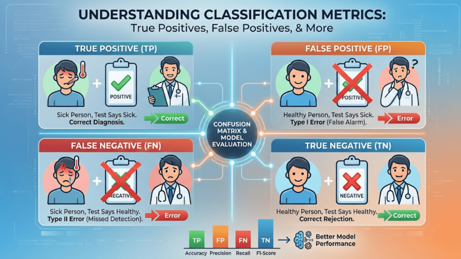
In binary classification, every prediction falls into one of four categories: a True Positive (TP) is a correct positive prediction, a True Negative (TN) is a correct negative prediction, a False Positive (FP) is an incorrect positive prediction (the model said “yes” but the truth was “no”), and a False Negative (FN) is an incorrect negative prediction (the model said “no” but the truth was “yes”). These four values form the confusion matrix, the foundation of almost every classification evaluation metric.
Introduction
Imagine you are developing a security system that screens airport luggage for dangerous items. The system can either flag a bag as suspicious (positive) or clear it as safe (negative). When it works correctly, it catches real threats and clears innocent travelers. But it also makes mistakes in two very different ways: it sometimes raises a false alarm on a harmless bag (wasting everyone’s time), and it sometimes misses an actual threat entirely (a potentially catastrophic failure).
These two types of mistakes have dramatically different consequences. Yet a single metric like accuracy treats them as identical. To build systems that behave correctly in the real world, you need to understand all four possible outcomes of a binary classifier’s predictions — and you need to understand them deeply, not just as abstract terms.
This article provides that deep understanding. We will work through every one of the four fundamental prediction outcomes with multiple real-world examples, build intuition for when each type of error matters, explore how they combine into the confusion matrix, and implement everything in Python. By the time you finish, these concepts will feel completely natural — and you will understand why the choice of what to optimize for is often the most consequential decision in machine learning.
The Binary Classification Setting
Before we define the four terms, let’s establish the context clearly.
In binary classification, every sample in your dataset belongs to one of exactly two classes. We conventionally call these:
- The positive class: the class of primary interest, what we are looking for. Examples: disease present, email is spam, transaction is fraudulent, item is defective.
- The negative class: the absence of the thing we’re looking for. Examples: disease absent, email is legitimate, transaction is legitimate, item is fine.
The naming is a convention. “Positive” doesn’t mean good or desirable — it simply means “the thing the test is designed to detect.” Cancer screening tests for cancer (positive = cancer present). Spam filters test for spam (positive = email is spam). Fraud detectors test for fraud (positive = transaction is fraudulent).
Your trained classifier takes an input sample and outputs a prediction: positive or negative. There are only four possible combinations of (actual truth, model prediction):
The Four Fundamental Outcomes
True Positive (TP)
Definition: The model predicts positive, and the actual label is positive. The prediction is correct.
The “True” part means the prediction is correct — the model said positive and was right. The “Positive” part refers to what the model predicted.
Real-world examples:
- Medical diagnosis: The cancer screening test flags a patient as having cancer (positive), and the follow-up biopsy confirms cancer is present. The test was right. This is a TP.
- Spam filter: The filter classifies an email as spam (positive), and it really is spam. The filter was right. This is a TP.
- Fraud detection: The fraud model flags a transaction as fraudulent (positive), and the bank investigation confirms fraud occurred. This is a TP.
- Airport security: The scanner flags a bag as suspicious (positive), and officers find a prohibited item inside. This is a TP.
True positives represent the classifier’s successes on the class it cares about most. More TPs means the model is finding more real cases of what it’s looking for.
True Negative (TN)
Definition: The model predicts negative, and the actual label is negative. The prediction is correct.
The “True” part means the prediction is correct — the model said negative and was right. The “Negative” part refers to what the model predicted.
Real-world examples:
- Medical diagnosis: The cancer screening test clears a patient as healthy (negative), and the patient actually is healthy. The test correctly identified no cancer. This is a TN.
- Spam filter: The filter lets an email through as legitimate (negative), and it really is a legitimate email from a colleague. This is a TN.
- Fraud detection: The fraud model lets a purchase through as legitimate (negative), and it really is a legitimate grocery shopping trip. This is a TN.
- Airport security: The scanner clears a bag (negative), and officers confirm it contains only clothes and toiletries. This is a TN.
True negatives represent the classifier’s successes on the majority class. In most real-world problems, the negative class is by far the larger class (most patients are healthy, most emails are legitimate, most transactions are not fraud), so TNs tend to dominate the confusion matrix. This is exactly why accuracy can be misleading — a model that outputs only TNs appears very accurate.
False Positive (FP) — The Type I Error
Definition: The model predicts positive, but the actual label is negative. The prediction is incorrect — a false alarm.
The “False” part means the prediction is wrong — the model said positive but was wrong. The “Positive” part refers to what the model predicted (incorrectly).
The false positive is also called a Type I error in statistical hypothesis testing, or a false alarm.
Real-world examples:
- Medical diagnosis: The cancer screening test flags a healthy patient as having cancer. The patient undergoes an unnecessary (and potentially harmful) biopsy, experiences intense anxiety, and is eventually told the result was wrong. This is a FP.
- Spam filter: The filter sends a critical business email to the spam folder. The user misses an important meeting invitation. This is a FP.
- Fraud detection: The fraud system blocks a legitimate credit card transaction, embarrassing the cardholder at the checkout counter and requiring a phone call to unblock the card. This is a FP.
- Airport security: Security flags and searches a traveler whose bag contains only harmless personal items. The traveler misses their flight. This is a FP.
The cost of false positives varies enormously by application. In spam filtering, a FP is annoying. In medical diagnostics, a FP causes unnecessary procedures and psychological harm. In criminal justice applications, a FP could mean an innocent person is treated as a suspect.
False Negative (FN) — The Type II Error
Definition: The model predicts negative, but the actual label is positive. The prediction is incorrect — a miss.
The “False” part means the prediction is wrong — the model said negative but was wrong. The “Negative” part refers to what the model predicted (incorrectly).
The false negative is also called a Type II error in statistical hypothesis testing, or a miss.
Real-world examples:
- Medical diagnosis: The cancer screening test clears a patient as healthy, but the patient actually has early-stage cancer. Because of the miss, they receive no treatment during the critical window when cancer is most treatable. This is a FN — and potentially fatal.
- Spam filter: The filter lets a phishing email through to the inbox, and the user clicks the link and has their credentials stolen. This is a FN.
- Fraud detection: The fraud system approves a fraudulent transaction, and the stolen money is transferred before anyone notices. This is a FN.
- Airport security: The scanner clears a bag containing a prohibited item, and that item makes it onto a flight. This is a FN — and potentially catastrophic.
The cost of false negatives also varies enormously. Missing a spam email is trivial. Missing a cancer case can be fatal. Missing a fraudulent transaction costs money. Missing a security threat can endanger lives.
The Confusion Matrix: Organizing All Four Outcomes
The confusion matrix arranges all four outcomes in a 2×2 table. The standard convention places actual values in rows and predicted values in columns:
| Predicted Positive | Predicted Negative | |
|---|---|---|
| Actual Positive | True Positive (TP) | False Negative (FN) |
| Actual Negative | False Positive (FP) | True Negative (TN) |
Every prediction made by your classifier falls exactly into one of these four cells. The cells along the main diagonal (top-left to bottom-right: TP and TN) represent correct predictions. The cells on the off-diagonal (top-right and bottom-left: FN and FP) represent incorrect predictions.
A perfect model would have all predictions on the main diagonal, with FP = 0 and FN = 0.
Reading the Confusion Matrix Correctly
Many beginners get confused about which axis is which. A helpful memory trick:
- Rows = Reality (what actually happened)
- Columns = Classifier’s claims (what the model said)
Or think of it as a trial: rows are what the defendant actually did (guilty/innocent), columns are the verdict (convicted/acquitted). The four cells then correspond to: correct conviction (TP), wrongful acquittal (FN), wrongful conviction (FP), correct acquittal (TN).
A Complete Numeric Example
Let’s work through a realistic example to make these concepts concrete.
A hospital deploys a machine learning model to screen patients for early-stage Type 2 diabetes. They test it on 1,000 patients and compare the model’s predictions to confirmed diagnoses:
- 200 patients truly have diabetes (actual positives)
- 800 patients do not have diabetes (actual negatives)
The model produces these results:
| Predicted: Diabetic | Predicted: Not Diabetic | Total | |
|---|---|---|---|
| Actually Diabetic | 160 (TP) | 40 (FN) | 200 |
| Actually Not Diabetic | 60 (FP) | 740 (TN) | 800 |
| Total | 220 | 780 | 1,000 |
Let’s unpack what each cell means:
TP = 160: The model correctly identified 160 patients who actually have diabetes. These patients will receive early treatment.
FN = 40: The model missed 40 diabetes patients, clearing them as healthy. These patients will not receive timely treatment. This is a medically serious error.
FP = 60: The model incorrectly flagged 60 healthy patients as diabetic. These patients will undergo unnecessary follow-up tests, experience anxiety, and face potential misdiagnosis.
TN = 740: The model correctly cleared 740 healthy patients. These patients are correctly dismissed.
Accuracy: (160 + 740) / 1000 = 90% — looks excellent on the surface.
But look more carefully: 40 out of 200 diabetes patients were missed (20% miss rate). And 60 healthy patients were incorrectly flagged (7.5% false alarm rate). Whether 90% accuracy is acceptable depends entirely on how you weigh these two types of errors against each other.
The Asymmetry of Errors: Why Both Types Matter Differently
The most important insight about FPs and FNs is that their costs are rarely equal. The relative cost of each error type defines what your model should optimize for.
The Cost Matrix Framework
In decision theory, the cost matrix makes error costs explicit:
| Predicted Positive | Predicted Negative | |
|---|---|---|
| Actual Positive | Cost(TP) — often 0 or reward | Cost(FN) — miss |
| Actual Negative | Cost(FP) — false alarm | Cost(TN) — often 0 |
For the diabetes screening example:
- Cost(FN): Patient with undiagnosed diabetes proceeds without treatment. Risk of complications, hospitalization, long-term damage. Estimated cost: high (measured in patient health and healthcare expense).
- Cost(FP): Healthy patient undergoes follow-up blood tests (HbA1c, oral glucose tolerance test). Cost: relatively low (a few hundred dollars and some inconvenience).
Since Cost(FN) >> Cost(FP), the diabetes screening model should be tuned to prioritize high recall (catching more TPs even at the cost of more FPs).
Asymmetric Cost Examples Across Domains
| Domain | FP Consequence | FN Consequence | Optimize For |
|---|---|---|---|
| Cancer screening | Unnecessary biopsy (uncomfortable, costly) | Missed early cancer (potentially fatal) | Recall (minimize FN) |
| Spam filtering | Lost legitimate email (annoying) | Spam in inbox (minor irritation) | Precision (minimize FP) |
| Fraud detection | Blocked legitimate transaction (frustrating) | Money stolen (financial loss) | Recall (minimize FN) |
| Nuclear plant alarm | Unnecessary evacuation (costly, disruptive) | Missed critical failure (catastrophic) | Recall (minimize FN) |
| Drug testing athletes | Innocent athlete banned (career-ending) | Cheating goes undetected (unfair) | Precision (minimize FP) |
| Search engine | Irrelevant result shown (poor UX) | Relevant result missed (poor UX) | Precision (minimize FP) |
| COVID-19 testing | Person quarantines unnecessarily | Infected person spreads disease | Recall (minimize FN) |
Python Implementation: Building and Analyzing the Confusion Matrix
From Scratch
import numpy as np
import matplotlib.pyplot as plt
import seaborn as sns
from collections import namedtuple

ConfusionValues = namedtuple('ConfusionValues', ['TP', 'FP', 'FN', 'TN'])

def compute_confusion_values(y_true, y_pred, positive_label=1):
    """
    Compute TP, FP, FN, TN from true and predicted labels.

    Args:
        y_true:         Array of true labels
        y_pred:         Array of predicted labels
        positive_label: Which label is the 'positive' class (default: 1)

    Returns:
        ConfusionValues namedtuple with TP, FP, FN, TN
    """
    y_true = np.array(y_true)
    y_pred = np.array(y_pred)

    TP = int(np.sum((y_true == positive_label) & (y_pred == positive_label)))
    FP = int(np.sum((y_true != positive_label) & (y_pred == positive_label)))
    FN = int(np.sum((y_true == positive_label) & (y_pred != positive_label)))
    TN = int(np.sum((y_true != positive_label) & (y_pred != positive_label)))

    return ConfusionValues(TP=TP, FP=FP, FN=FN, TN=TN)


def confusion_matrix_report(y_true, y_pred, class_names=("Negative", "Positive")):
    """
    Print a complete confusion matrix report with all derived metrics.
    """
    cv = compute_confusion_values(y_true, y_pred)
    n_total = cv.TP + cv.FP + cv.FN + cv.TN
    n_actual_pos = cv.TP + cv.FN
    n_actual_neg = cv.FP + cv.TN
    n_pred_pos   = cv.TP + cv.FP
    n_pred_neg   = cv.FN + cv.TN

    print("=" * 52)
    print("  CONFUSION MATRIX REPORT")
    print("=" * 52)

    # Visual matrix
    print(f"\n  {'':20} {'Pred: ' + class_names[1]:>15} {'Pred: ' + class_names[0]:>15}")
    print(f"  {'Actual: ' + class_names[1]:<20} {cv.TP:>15,} {cv.FN:>15,}   ← actual positives: {n_actual_pos:,}")
    print(f"  {'Actual: ' + class_names[0]:<20} {cv.FP:>15,} {cv.TN:>15,}   ← actual negatives: {n_actual_neg:,}")
    print(f"  {'':20} {'↑':>15} {'↑':>15}")
    print(f"  {'':20} {f'pred pos: {n_pred_pos}':>15} {f'pred neg: {n_pred_neg}':>15}")

    print(f"\n  Total samples: {n_total:,}")
    print(f"  TP: {cv.TP:,}  |  FP: {cv.FP:,}  |  FN: {cv.FN:,}  |  TN: {cv.TN:,}")

    # Core metrics (with division-by-zero guards)
    accuracy  = (cv.TP + cv.TN) / n_total if n_total > 0 else 0
    precision = cv.TP / (cv.TP + cv.FP) if (cv.TP + cv.FP) > 0 else 0
    recall    = cv.TP / (cv.TP + cv.FN) if (cv.TP + cv.FN) > 0 else 0
    f1        = 2 * precision * recall / (precision + recall) if (precision + recall) > 0 else 0
    specificity = cv.TN / (cv.TN + cv.FP) if (cv.TN + cv.FP) > 0 else 0
    npv       = cv.TN / (cv.TN + cv.FN) if (cv.TN + cv.FN) > 0 else 0  # Negative Predictive Value
    fpr       = cv.FP / (cv.FP + cv.TN) if (cv.FP + cv.TN) > 0 else 0
    fnr       = cv.FN / (cv.FN + cv.TP) if (cv.FN + cv.TP) > 0 else 0

    print(f"\n  Derived Metrics:")
    print(f"  {'Accuracy':<30} {accuracy:.4f}  ({accuracy*100:.1f}%)")
    print(f"  {'Precision (PPV)':<30} {precision:.4f}  of predicted pos, how many are real pos")
    print(f"  {'Recall (Sensitivity / TPR)':<30} {recall:.4f}  of actual pos, how many we caught")
    print(f"  {'Specificity (TNR)':<30} {specificity:.4f}  of actual neg, how many we cleared")
    print(f"  {'F1 Score':<30} {f1:.4f}  harmonic mean of precision & recall")
    print(f"  {'NPV (Neg Predictive Value)':<30} {npv:.4f}  of predicted neg, how many are real neg")
    print(f"  {'FPR (False Positive Rate)':<30} {fpr:.4f}  of actual neg, how many we wrongly flagged")
    print(f"  {'FNR (False Negative Rate)':<30} {fnr:.4f}  of actual pos, how many we missed")

    return cv


# Apply to the diabetes example
print("=== Diabetes Screening Model ===\n")
# Build y_true and y_pred from our confusion matrix values
y_true_diabetes = np.array([1]*200 + [0]*800)
y_pred_diabetes = np.array([1]*160 + [0]*40 +   # 160 TP, 40 FN (actual positives)
                            [1]*60  + [0]*740)    # 60 FP, 740 TN (actual negatives)

cv = confusion_matrix_report(y_true_diabetes, y_pred_diabetes,
class_names=("Not Diabetic", "Diabetic"))Visualizing the Confusion Matrix
def plot_confusion_matrix_detailed(y_true, y_pred,
                                    class_names=("Negative", "Positive"),
                                    title="Confusion Matrix",
                                    cmap="Blues"):
    """
    Create a detailed, annotated confusion matrix heatmap.
    Shows both raw counts and percentages for easy interpretation.
    """
    from sklearn.metrics import confusion_matrix

    cm = confusion_matrix(y_true, y_pred)
    cm_percent = cm.astype(float) / cm.sum(axis=1, keepdims=True) * 100

    fig, axes = plt.subplots(1, 2, figsize=(14, 5))

    # Panel 1: Raw counts
    sns.heatmap(cm, annot=True, fmt='d', cmap=cmap, ax=axes[0],
                xticklabels=[f"Pred:\n{c}" for c in class_names],
                yticklabels=[f"Actual:\n{c}" for c in class_names],
                cbar=False, linewidths=2, linecolor='white',
                annot_kws={"size": 16, "weight": "bold"})
    axes[0].set_title(f"{title}\n(Raw Counts)", fontsize=13, fontweight='bold')
    axes[0].set_ylabel("Actual Class", fontsize=11)
    axes[0].set_xlabel("Predicted Class", fontsize=11)

    # Add TP/FP/FN/TN labels
    cell_labels = [["TN", "FP"], ["FN", "TP"]]
    for i in range(2):
        for j in range(2):
            axes[0].text(j + 0.5, i + 0.75, cell_labels[i][j],
                        ha='center', va='center', fontsize=11,
                        color='white' if cm[i, j] > cm.max() * 0.5 else 'gray',
                        alpha=0.8)

    # Panel 2: Row-normalized percentages (what % of each actual class)
    annot_text = np.array([[f"{cm[i,j]}\n({cm_percent[i,j]:.1f}%)"
                            for j in range(2)] for i in range(2)])

    sns.heatmap(cm_percent, annot=annot_text, fmt='', cmap=cmap, ax=axes[1],
                xticklabels=[f"Pred:\n{c}" for c in class_names],
                yticklabels=[f"Actual:\n{c}" for c in class_names],
                vmin=0, vmax=100, cbar=True, linewidths=2, linecolor='white',
                annot_kws={"size": 12})
    axes[1].set_title(f"{title}\n(Row-Normalized %)", fontsize=13, fontweight='bold')
    axes[1].set_ylabel("Actual Class", fontsize=11)
    axes[1].set_xlabel("Predicted Class", fontsize=11)

    plt.suptitle("The confusion matrix shows all four prediction outcome types",
                 fontsize=11, style='italic', y=0)
    plt.tight_layout()
    plt.savefig("confusion_matrix_detailed.png", dpi=150, bbox_inches='tight')
    plt.show()
    print("Saved: confusion_matrix_detailed.png")

plot_confusion_matrix_detailed(y_true_diabetes, y_pred_diabetes,
                                class_names=("Not Diabetic", "Diabetic"),
title="Diabetes Screening Model")All Derived Metrics from TP, FP, FN, TN
Every classification metric is derived from these four numbers. Understanding the derivation makes the metrics intuitive rather than memorized formulas.
The Complete Metric Family
def all_metrics_from_confusion(TP, FP, FN, TN):
    """
    Compute every standard classification metric from the four confusion values.

    This function makes explicit how all metrics derive from TP, FP, FN, TN.
    """
    total = TP + FP + FN + TN
    actual_pos  = TP + FN
    actual_neg  = FP + TN
    pred_pos    = TP + FP
    pred_neg    = FN + TN

    def safe_div(a, b):
        return a / b if b > 0 else 0.0

    metrics = {}

    # --- Accuracy family ---
    metrics["Accuracy"]           = safe_div(TP + TN, total)
    metrics["Error Rate"]         = safe_div(FP + FN, total)   # = 1 - Accuracy
    metrics["Balanced Accuracy"]  = 0.5 * (safe_div(TP, actual_pos) + safe_div(TN, actual_neg))

    # --- Positive prediction quality ---
    metrics["Precision (PPV)"]    = safe_div(TP, pred_pos)      # Of all predicted +, how many are real +?
    metrics["Recall (TPR/Sens)"]  = safe_div(TP, actual_pos)    # Of all actual +, how many did we catch?
    metrics["F1 Score"]           = safe_div(2 * TP, 2*TP + FP + FN)
    metrics["F2 Score"]           = safe_div(5 * TP, 5*TP + 4*FN + FP)  # Recall-weighted

    # --- Negative prediction quality ---
    metrics["Specificity (TNR)"]  = safe_div(TN, actual_neg)    # Of all actual -, how many did we clear?
    metrics["NPV"]                = safe_div(TN, pred_neg)      # Of all predicted -, how many are real -?

    # --- Error rates ---
    metrics["FPR (Fall-out)"]     = safe_div(FP, actual_neg)    # = 1 - Specificity
    metrics["FNR (Miss Rate)"]    = safe_div(FN, actual_pos)    # = 1 - Recall
    metrics["FDR (False Disc.)"]  = safe_div(FP, pred_pos)      # = 1 - Precision
    metrics["FOR (False Omit.)"]  = safe_div(FN, pred_neg)      # = 1 - NPV

    # --- Composite ---
    mcc_denom = np.sqrt(pred_pos * pred_neg * actual_pos * actual_neg)
    metrics["MCC (Matthews CC)"]  = safe_div(TP*TN - FP*FN, mcc_denom) if mcc_denom > 0 else 0

    return metrics


# Apply to our diabetes model
print("\n=== All Metrics from the Diabetes Model ===\n")
metrics = all_metrics_from_confusion(TP=160, FP=60, FN=40, TN=740)

print(f"  {'Metric':<28} | {'Value':>8} | Meaning")
print("-" * 80)

metric_meanings = {
    "Accuracy":          "Overall correct predictions",
    "Error Rate":        "Overall incorrect predictions",
    "Balanced Accuracy": "Average of TPR and TNR (good for imbalanced data)",
    "Precision (PPV)":   "Of patients flagged as diabetic, 72.7% actually are",
    "Recall (TPR/Sens)": "Of actual diabetics, 80% were correctly identified",
    "F1 Score":          "Harmonic mean of precision and recall",
    "F2 Score":          "F1 weighted toward recall (good for medical screening)",
    "Specificity (TNR)": "Of healthy patients, 92.5% were correctly cleared",
    "NPV":               "Of patients cleared as healthy, 94.9% actually are healthy",
    "FPR (Fall-out)":    "7.5% of healthy patients were wrongly flagged",
    "FNR (Miss Rate)":   "20% of diabetics were wrongly cleared — missed!",
    "FDR (False Disc.)": "27.3% of 'diabetic' predictions are actually healthy",
    "FOR (False Omit.)": "5.1% of 'healthy' predictions are actually diabetic",
    "MCC (Matthews CC)": "Comprehensive measure; +1=perfect, 0=random, -1=inverse",
}

for name, value in metrics.items():
    meaning = metric_meanings.get(name, "")
print(f" {name:<28} | {value:>8.4f} | {meaning}")The Metric Relationships Map
All metrics form a connected web. Here is how they relate:
TP, FP, FN, TN
    │
    ├─ Accuracy       = (TP + TN) / N
    ├─ Precision      = TP / (TP + FP)           → FDR = 1 - Precision
    ├─ Recall (TPR)   = TP / (TP + FN)           → FNR = 1 - Recall
    ├─ Specificity    = TN / (TN + FP)           → FPR = 1 - Specificity
    ├─ NPV            = TN / (TN + FN)           → FOR = 1 - NPV
    ├─ F1             = 2×Precision×Recall / (P+R)
└─ MCC = (TP×TN - FP×FN) / √(...)The Impact of Threshold on All Four Values
Classifiers typically output a probability score, and you apply a threshold to convert it to a binary label. As you move the threshold, all four confusion matrix values change simultaneously.
from sklearn.datasets import make_classification
from sklearn.linear_model import LogisticRegression
from sklearn.model_selection import train_test_split
import numpy as np
import matplotlib.pyplot as plt

# Generate classification data
np.random.seed(42)
X, y = make_classification(
    n_samples=1000, n_features=10, n_informative=6,
    weights=[0.8, 0.2], random_state=42  # 80% negative, 20% positive
)

X_train, X_test, y_train, y_test = train_test_split(X, y, test_size=0.3,
                                                     stratify=y, random_state=42)

model = LogisticRegression(random_state=42, max_iter=1000)
model.fit(X_train, y_train)
y_proba = model.predict_proba(X_test)[:, 1]

# Track TP, FP, FN, TN at each threshold
thresholds = np.linspace(0.01, 0.99, 100)
tp_vals, fp_vals, fn_vals, tn_vals = [], [], [], []

for t in thresholds:
    y_pred_t = (y_proba >= t).astype(int)
    cv = compute_confusion_values(y_test, y_pred_t)
    tp_vals.append(cv.TP)
    fp_vals.append(cv.FP)
    fn_vals.append(cv.FN)
    tn_vals.append(cv.TN)

# Plot
fig, axes = plt.subplots(2, 2, figsize=(14, 10))

plot_data = [
    (axes[0,0], tp_vals, 'TP', 'mediumseagreen', 'True Positives\n(correctly caught positive cases)'),
    (axes[0,1], tn_vals, 'TN', 'steelblue',      'True Negatives\n(correctly cleared negative cases)'),
    (axes[1,0], fp_vals, 'FP', 'coral',           'False Positives\n(wrongly flagged negative cases)'),
    (axes[1,1], fn_vals, 'FN', 'mediumpurple',    'False Negatives\n(missed positive cases)'),
]

for ax, vals, label, color, full_label in plot_data:
    ax.plot(thresholds, vals, color=color, linewidth=2.5)
    ax.axvline(x=0.5, color='gray', linestyle='--', alpha=0.7, label='Default threshold (0.5)')
    ax.set_xlabel("Decision Threshold", fontsize=11)
    ax.set_ylabel("Count", fontsize=11)
    ax.set_title(f"{label}: {full_label}", fontsize=11, fontweight='bold')
    ax.legend(fontsize=9)
    ax.grid(True, alpha=0.3)

plt.suptitle("How TP, TN, FP, FN Change as the Decision Threshold Moves",
             fontsize=13, fontweight='bold', y=1.01)
plt.tight_layout()
plt.savefig("threshold_vs_confusion_values.png", dpi=150, bbox_inches='tight')
plt.show()
print("Saved: threshold_vs_confusion_values.png")

# Print values at selected thresholds
print(f"\n{'Threshold':>10} | {'TP':>6} | {'FP':>6} | {'FN':>6} | {'TN':>6} | {'Precision':>10} | {'Recall':>7}")
print("-" * 70)
for t in [0.2, 0.3, 0.4, 0.5, 0.6, 0.7, 0.8]:
    y_pred_t = (y_proba >= t).astype(int)
    cv = compute_confusion_values(y_test, y_pred_t)
    prec = cv.TP / (cv.TP + cv.FP) if (cv.TP + cv.FP) > 0 else 0
    rec  = cv.TP / (cv.TP + cv.FN) if (cv.TP + cv.FN) > 0 else 0
print(f"{t:>10.1f} | {cv.TP:>6} | {cv.FP:>6} | {cv.FN:>6} | {cv.TN:>6} | {prec:>10.4f} | {rec:>7.4f}")Lowering the threshold increases TP and FP while decreasing FN and TN. Raising it decreases TP and FP while increasing FN and TN. This is the fundamental precision-recall tradeoff expressed directly in confusion matrix terms.
Multiclass Confusion Matrices
Real-world problems often have more than two classes. The confusion matrix extends naturally to any number of classes, becoming an N×N matrix.
from sklearn.metrics import confusion_matrix, classification_report
import numpy as np
import matplotlib.pyplot as plt
import seaborn as sns

# Three-class example: medical triage
# Classes: 0=Low Risk, 1=Medium Risk, 2=High Risk
y_true_multi = np.array([0]*50 + [1]*30 + [2]*20)  # 50 low, 30 medium, 20 high risk

# Simulated model predictions (with some realistic errors)
np.random.seed(42)
y_pred_multi = np.array([
    # Low risk: mostly correct, some confused with medium
    *np.random.choice([0, 1], size=50, p=[0.88, 0.12]),
    # Medium risk: often confused with both low and high
    *np.random.choice([0, 1, 2], size=30, p=[0.10, 0.70, 0.20]),
    # High risk: mostly correct, some confused with medium
    *np.random.choice([1, 2], size=20, p=[0.15, 0.85]),
])

class_names = ["Low Risk", "Medium Risk", "High Risk"]
cm_multi = confusion_matrix(y_true_multi, y_pred_multi)

# Plot multiclass confusion matrix
plt.figure(figsize=(8, 6))
sns.heatmap(cm_multi, annot=True, fmt='d', cmap='Blues',
            xticklabels=[f"Pred:\n{c}" for c in class_names],
            yticklabels=[f"Actual:\n{c}" for c in class_names],
            linewidths=2, linecolor='white',
            annot_kws={"size": 14, "weight": "bold"})
plt.title("Multiclass Confusion Matrix\n(Medical Triage: 3 Risk Levels)",
          fontsize=13, fontweight='bold')
plt.ylabel("Actual Class", fontsize=11)
plt.xlabel("Predicted Class", fontsize=11)
plt.tight_layout()
plt.savefig("multiclass_confusion_matrix.png", dpi=150)
plt.show()

print("\n=== Multiclass Classification Report ===\n")
print(classification_report(y_true_multi, y_pred_multi, target_names=class_names))

# In multiclass, TP/FP/FN/TN are computed per class using One-vs-Rest
print("=== Per-Class TP, FP, FN, TN (One-vs-Rest) ===\n")
print(f"{'Class':<14} | {'TP':>5} | {'FP':>5} | {'FN':>5} | {'TN':>5} | {'Precision':>10} | {'Recall':>7}")
print("-" * 65)

for i, class_name in enumerate(class_names):
    # Binarize: this class = positive, all others = negative
    y_true_bin = (y_true_multi == i).astype(int)
    y_pred_bin = (y_pred_multi == i).astype(int)

    cv = compute_confusion_values(y_true_bin, y_pred_bin)
    prec = cv.TP / (cv.TP + cv.FP) if (cv.TP + cv.FP) > 0 else 0
    rec  = cv.TP / (cv.TP + cv.FN) if (cv.TP + cv.FN) > 0 else 0

    print(f"{class_name:<14} | {cv.TP:>5} | {cv.FP:>5} | {cv.FN:>5} | {cv.TN:>5} | "
f"{prec:>10.4f} | {rec:>7.4f}")Real-World Case Study: Building a COVID-19 Screening Tool
Let’s put everything together with a realistic case study that demonstrates how to reason about all four confusion matrix values in a high-stakes setting.
import numpy as np
from sklearn.datasets import make_classification
from sklearn.linear_model import LogisticRegression
from sklearn.ensemble import RandomForestClassifier
from sklearn.model_selection import train_test_split
from sklearn.metrics import confusion_matrix
import warnings
warnings.filterwarnings('ignore')

# --------------------------------------------------------
# Scenario: COVID-19 rapid screening at an airport
# Population: 10,000 travelers
# True prevalence: 2% (200 infected, 9,800 healthy)
# Goal: Identify infected travelers for quarantine
# --------------------------------------------------------

np.random.seed(42)
n = 10000
prevalence = 0.02

# Simulate clinical features (symptoms, travel history, etc.)
X, y = make_classification(
    n_samples=n,
    n_features=12,
    n_informative=8,
    weights=[1 - prevalence, prevalence],
    random_state=42,
    flip_y=0.02
)

X_train, X_test, y_train, y_test = train_test_split(
    X, y, test_size=0.3, random_state=42, stratify=y
)

# Train two models
lr_model = LogisticRegression(class_weight='balanced', random_state=42, max_iter=1000)
rf_model = RandomForestClassifier(100, class_weight='balanced', random_state=42)

lr_model.fit(X_train, y_train)
rf_model.fit(X_train, y_train)

y_proba_lr = lr_model.predict_proba(X_test)[:, 1]
y_proba_rf = rf_model.predict_proba(X_test)[:, 1]

def evaluate_screening_model(y_true, y_proba, model_name, threshold=0.5):
    """
    Evaluate a COVID screening model with full cost analysis.
    """
    y_pred = (y_proba >= threshold).astype(int)
    cv = compute_confusion_values(y_true, y_pred)

    n_total     = cv.TP + cv.FP + cv.FN + cv.TN
    prevalence  = (cv.TP + cv.FN) / n_total

    precision   = cv.TP / (cv.TP + cv.FP) if (cv.TP + cv.FP) > 0 else 0
    recall      = cv.TP / (cv.TP + cv.FN) if (cv.TP + cv.FN) > 0 else 0
    specificity = cv.TN / (cv.TN + cv.FP) if (cv.TN + cv.FP) > 0 else 0

    # Real-world cost estimation
    cost_per_fp = 500    # Quarantine healthy person: hotel, lost wages, testing
    cost_per_fn = 50000  # Infected person spreads disease: estimated societal cost

    total_cost = cv.FP * cost_per_fp + cv.FN * cost_per_fn

    print(f"\n{'='*55}")
    print(f"  {model_name} (threshold={threshold})")
    print(f"{'='*55}")
    print(f"  Total travelers screened: {n_total:,}")
    print(f"  Actually infected:        {cv.TP + cv.FN:,} ({prevalence*100:.1f}%)")
    print(f"\n  Confusion Matrix:")
    print(f"    TP (caught infections):    {cv.TP:>5,}  ← quarantine, protect others")
    print(f"    FN (missed infections):    {cv.FN:>5,}  ← board plane, risk spreading")
    print(f"    FP (healthy quarantined):  {cv.FP:>5,}  ← unnecessary quarantine")
    print(f"    TN (healthy cleared):      {cv.TN:>5,}  ← board plane safely")
    print(f"\n  Performance:")
    print(f"    Recall (catch rate):       {recall:.2%}  — caught {recall*100:.1f}% of infections")
    print(f"    Precision:                 {precision:.2%}  — {precision*100:.1f}% of quarantines are real")
    print(f"    Specificity:               {specificity:.2%}  — {specificity*100:.1f}% of healthy travelers cleared")
    print(f"\n  Cost Analysis (estimates):")
    print(f"    FP cost (@${cost_per_fp}/person):    ${cv.FP * cost_per_fp:>10,.0f}")
    print(f"    FN cost (@${cost_per_fn}/person):  ${cv.FN * cost_per_fn:>10,.0f}")
    print(f"    Total estimated cost:          ${total_cost:>10,.0f}")

    return {"model": model_name, "threshold": threshold,
            "TP": cv.TP, "FP": cv.FP, "FN": cv.FN, "TN": cv.TN,
            "recall": recall, "precision": precision, "cost": total_cost}


print("=== COVID-19 Airport Screening Evaluation ===")

# Default threshold
r1 = evaluate_screening_model(y_test, y_proba_lr, "Logistic Regression", threshold=0.5)
r2 = evaluate_screening_model(y_test, y_proba_rf, "Random Forest", threshold=0.5)

# High-recall threshold (public health priority: catch every infection)
print("\n\n--- Public Health Priority: Minimize FN (threshold=0.2) ---")
r3 = evaluate_screening_model(y_test, y_proba_rf, "Random Forest (High Recall)", threshold=0.2)

# Show the tradeoff
print("\n\n=== Threshold Tradeoff Summary ===\n")
print(f"{'Setting':<35} | {'TP':>4} | {'FP':>5} | {'FN':>4} | {'Recall':>7} | {'Cost':>12}")
print("-" * 80)
for r in [r1, r2, r3]:
    print(f"{r['model']:<35} | {r['TP']:>4} | {r['FP']:>5} | {r['FN']:>4} | "
          f"{r['recall']:>7.2%} | ${r['cost']:>11,.0f}")

print("\nConclusion: Lower threshold catches more infections (↑TP, ↓FN)")
print("but quarantines more healthy travelers (↑FP). Cost analysis guides the tradeoff.")Common Misconceptions and Pitfalls
Misconception 1: Accuracy Captures the Full Picture
The most common mistake. A model with 99% accuracy on fraud detection that catches 0 fraudulent transactions has TP = 0. All 99% accuracy comes from correct negative predictions. The confusion matrix immediately reveals this; accuracy alone never would.
Misconception 2: FP and FN Are Equally Bad
Almost never true in practice. Always reason about the specific costs of each error type in your domain before choosing a metric or setting a threshold.
Misconception 3: Reducing One Type of Error Doesn’t Affect the Other
Lowering the classification threshold to reduce FNs (catch more positives) always increases FPs simultaneously. There is no free lunch — only tradeoffs. The confusion matrix makes these tradeoffs visible.
Misconception 4: The “Positive” Class Is Always the Majority Class
No. The positive class is whichever class your detector is designed to find, regardless of its frequency. In fraud detection, fraud is positive even though it represents less than 0.1% of transactions.
Misconception 5: Confusion Matrix Values Are Fixed for a Trained Model
Wrong. For a model that outputs probabilities, the confusion matrix values change every time you change the decision threshold. Only the ROC curve and AUC are truly threshold-independent characterizations of model quality.
Practical Checklist for Confusion Matrix Analysis
Use this checklist whenever you evaluate a classification model:
Step 1: Establish your positive class explicitly. What is the “thing” your model is designed to detect? Make this explicit before computing anything.
Step 2: Compute and display the raw confusion matrix. Always look at absolute counts, not just rates. An FN rate of 5% on a dataset with 10,000 actual positives means 500 missed cases — that context matters.
Step 3: Calculate both FP rate and FN rate. These are the two types of mistakes. Report both — don’t hide one.
Step 4: Reason about the cost of each error type. For your specific application, which is worse: a false alarm or a missed detection? By how much?
Step 5: Choose your primary metric based on cost asymmetry. High FN cost → optimize recall. High FP cost → optimize precision. Both important → optimize F1 or Fbeta.
Step 6: Analyze the confusion matrix at your operating threshold. The default 0.5 threshold is almost never optimal. Compute the confusion matrix at your intended operating threshold, not just the default.
Step 7: For imbalanced data, check balanced accuracy or MCC. These capture both TP and TN performance even when class sizes differ dramatically.
Summary
True positives, false positives, true negatives, and false negatives are the atomic elements of classification evaluation. Every metric you will encounter — accuracy, precision, recall, F1, AUC, specificity, MCC — is ultimately derived from these four numbers.
Understanding them deeply, not just as formulas but as real-world outcomes with real consequences, is what separates a practitioner who can explain why their model behaves the way it does from one who can only report numbers. The confusion matrix makes these outcomes visible simultaneously, forcing you to confront the tradeoffs your model is making rather than hiding them behind a single aggregate score.
The most important practical lesson is the asymmetry of errors. In almost every real-world application, false positives and false negatives have different costs. Recognizing this, quantifying the difference, and building a model that optimizes for the right type of correctness is often the single most impactful decision in applied machine learning.