Underfitting vs Overfitting: Finding the Sweet Spot

Underfitting occurs when models are too simple to capture data patterns, resulting in poor performance on both training and test data. Overfitting happens when models are too complex, memorizing training data but failing on new data. The sweet spot—optimal model complexity—achieves good performance on both training and test data by learning true patterns without memorizing noise. Finding this balance requires monitoring performance curves, using validation sets, and adjusting model complexity systematically.

Introduction: The Goldilocks Problem of Machine Learning

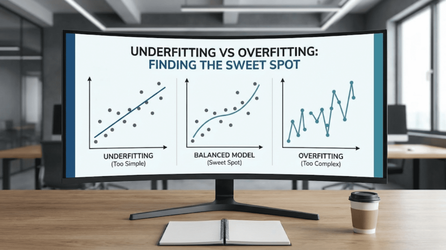
Remember the story of Goldilocks and the Three Bears? One bowl of porridge was too hot, another too cold, and one was just right. Machine learning faces an identical challenge with model complexity. Too simple, and your model underfits—failing to capture important patterns. Too complex, and it overfits—memorizing training data instead of learning generalizable patterns. The art of machine learning lies in finding the model that’s “just right.”

This balance between underfitting and overfitting isn’t just a theoretical concept—it’s the fundamental challenge that determines whether your model succeeds or fails in production. A severely underfit model is useless, barely better than random guessing. An overfit model looks impressive during development but crashes when deployed, having learned nothing useful about the actual problem.

Real-world machine learning projects constantly navigate this tradeoff. Data scientists spend enormous time tuning model complexity: adjusting the number of layers in neural networks, limiting tree depth in random forests, selecting features, setting regularization strength. All these decisions revolve around one question: how complex should the model be?

Understanding underfitting and overfitting deeply—recognizing their symptoms, knowing their causes, and mastering techniques to find the optimal balance—is essential for building effective machine learning systems. This isn’t about memorizing definitions; it’s about developing the intuition to diagnose what’s wrong when models underperform and knowing which knobs to turn to fix it.

This comprehensive guide explores both extremes and the optimal middle ground. You’ll learn to recognize underfitting and overfitting, understand the spectrum of model complexity, master techniques for finding the sweet spot, and develop practical strategies for optimizing your models. Whether you’re debugging a poor-performing model or designing a new system from scratch, understanding this fundamental tradeoff is crucial.

Understanding Underfitting: Too Simple to Succeed

Underfitting occurs when a model is too simple to capture the underlying patterns in the data. The model lacks the capacity or flexibility to learn the true relationships between features and labels.

What Underfitting Looks Like

Performance Characteristics:

• Low training accuracy/high training error
• Low test accuracy/high test error
• Similar poor performance on both training and test sets
• Model fails to learn even obvious patterns

Example:

Linear model predicting house prices
Training R²: 0.45
Test R²: 0.43
Conclusion: Both scores are poor; model underfits

Linear model predicting house prices
Training R²: 0.45
Test R²: 0.43
Conclusion: Both scores are poor; model underfits

The model performs badly everywhere, suggesting it hasn’t captured the underlying relationships in the data.

Visual Understanding

Imagine predicting house prices based on square footage:

True Relationship: Non-linear curve (prices increase faster for larger houses)

Underfit Model: Straight line that poorly represents the curve

• Misses the curvature
• Systematic errors throughout the range
• Can’t capture the true pattern no matter how much training data you provide

Analogy: Using a ruler to trace a circle. The ruler is fundamentally too limited for the task.

Root Causes of Underfitting

Cause 1: Model Too Simple

Problem: Model architecture lacks capacity to represent complex patterns

Examples:

• Linear regression for clearly non-linear relationship
• Single-layer neural network for complex image recognition
• Very shallow decision tree for intricate decision boundaries

Real-World Example:

Problem: Predict customer churn (complex behavior)
Model: Logistic regression with 2 features (age, tenure)
Reality: Churn depends on dozens of factors and their interactions
Result: Model too simple, underfits

Problem: Predict customer churn (complex behavior)
Model: Logistic regression with 2 features (age, tenure)
Reality: Churn depends on dozens of factors and their interactions
Result: Model too simple, underfits

Cause 2: Insufficient Features

Problem: Important information not included in features

Example:

Predicting house prices using only:
- Number of bedrooms
Missing critical features:
- Location, square footage, condition, age, etc.
Result: Model can't perform well regardless of algorithm

Predicting house prices using only:
- Number of bedrooms
Missing critical features:
- Location, square footage, condition, age, etc.
Result: Model can't perform well regardless of algorithm

Principle: You can’t predict what you can’t measure. Missing key features guarantees underfitting.

Cause 3: Over-Regularization

Problem: Regularization penalty too strong, forcing model to be too simple

Example:

Neural network with very high dropout (90%)
Effect: Most neurons turned off, model can't learn
Result: Underfitting despite complex architecture

Neural network with very high dropout (90%)
Effect: Most neurons turned off, model can't learn
Result: Underfitting despite complex architecture

Regularization prevents overfitting but too much causes underfitting.

Cause 4: Training Insufficient

Problem: Model not trained long enough to learn patterns

Indicators:

• Training stopped too early
• Learning rate too low (learning progresses too slowly)
• Optimization hasn’t converged

Example:

Deep neural network trained for 5 epochs
Potential: Could achieve 90% accuracy with more training
Actual: 65% accuracy (stopped too soon)

Deep neural network trained for 5 epochs
Potential: Could achieve 90% accuracy with more training
Actual: 65% accuracy (stopped too soon)

Cause 5: Poor Feature Engineering

Problem: Features don’t effectively represent the problem

Example:

Predicting success in sports using only:
- Player height in millimeters (45,720)
- Player weight in milligrams (72,574,779)

Issues: 
- Wrong scale (huge numbers)
- Missing derived features (height/weight ratio)
- No normalization
Result: Model struggles to learn

Predicting success in sports using only:
- Player height in millimeters (45,720)
- Player weight in milligrams (72,574,779)

Issues: 
- Wrong scale (huge numbers)
- Missing derived features (height/weight ratio)
- No normalization
Result: Model struggles to learn

Symptoms and Diagnosis

How to Recognize Underfitting:

1. Training performance is poor: Model doesn’t even fit training data well
2. No improvement with more training: Extended training doesn’t help
3. Similar train/test performance: Both are bad (no generalization gap)
4. Simple decision boundaries: Visually too simplistic for the data
5. High bias in predictions: Systematic errors, predictions consistently off

Diagnostic Questions:

• Does the model perform poorly on training data?
• Are training and test errors both high and similar?
• Does the model fail to capture obvious patterns?
• Would a human easily outperform this model?

Example Diagnosis:

Spam classifier results:
Training accuracy: 58%
Test accuracy: 56%

Analysis:
- Both scores poor (barely better than random)
- Small gap between train/test (2%)
- Diagnosis: Underfitting
- Action needed: Increase model complexity

Spam classifier results:
Training accuracy: 58%
Test accuracy: 56%

Analysis:
- Both scores poor (barely better than random)
- Small gap between train/test (2%)
- Diagnosis: Underfitting
- Action needed: Increase model complexity

Understanding Overfitting: Too Complex for Good

Overfitting occurs when a model is too complex relative to the available data, learning noise and spurious patterns specific to the training set.

What Overfitting Looks Like

Performance Characteristics:

• High training accuracy/low training error
• Low test accuracy/high test error
• Large gap between training and test performance
• Model memorizes training data but doesn’t generalize

Example:

Deep neural network classifying images
Training accuracy: 99%
Test accuracy: 68%
Conclusion: Large gap (31%) indicates overfitting

Deep neural network classifying images
Training accuracy: 99%
Test accuracy: 68%
Conclusion: Large gap (31%) indicates overfitting

Visual Understanding

True Relationship: Smooth curve with natural variation

Overfit Model: Wiggly curve passing through every training point exactly

• Captures every random fluctuation
• Perfect fit to training data
• Terrible predictions on new data

Analogy: Memorizing specific exam questions vs. understanding concepts. You ace the practice test but fail the real exam with different questions.

Root Causes of Overfitting

Cause 1: Model Too Complex

Problem: Too many parameters relative to training data

Examples:

• 10-layer neural network for 1,000 training examples
• Decision tree with no depth limit (grows until each leaf has one example)
• Polynomial regression with degree 20 for 100 data points

Principle: With enough parameters, you can memorize any dataset.

Cause 2: Training Too Long

Problem: Continued training after learning genuine patterns

Pattern:

Epochs 1-20: Learning general patterns
Epochs 21-30: Optimal performance
Epochs 31-100: Memorizing training specifics

Epochs 1-20: Learning general patterns
Epochs 21-30: Optimal performance
Epochs 31-100: Memorizing training specifics

Validation performance peaks then declines while training performance keeps improving.

Cause 3: Insufficient Training Data

Problem: Not enough examples to constrain complex model

Example:

Model with 10,000 parameters
Training data: 500 examples
Result: 20 parameters per example → severe overfitting risk

Model with 10,000 parameters
Training data: 500 examples
Result: 20 parameters per example → severe overfitting risk

Rule of Thumb: Need 10-100x more examples than parameters (varies by problem).

Cause 4: Noisy Data

Problem: Model learns noise as if it’s signal

Example:

Data contains:
- Mislabeled examples (10%)
- Measurement errors
- Random variations
Complex model fits all of this noise
Result: Excellent training performance, poor generalization

Data contains:
- Mislabeled examples (10%)
- Measurement errors
- Random variations
Complex model fits all of this noise
Result: Excellent training performance, poor generalization

Cause 5: No Regularization

Problem: Nothing constrains model complexity

Example:

Model free to use all parameters fully
No penalty for complexity
Result: Overfits by using every parameter to fit noise

Model free to use all parameters fully
No penalty for complexity
Result: Overfits by using every parameter to fit noise

Symptoms and Diagnosis

How to Recognize Overfitting:

1. Large train-test gap: Training performance much better than test
2. Near-perfect training: 99-100% training accuracy suggests memorization
3. Degrading validation: Validation performance worsens over training time
4. Unstable predictions: Small data changes cause large prediction changes
5. Complex patterns: Decision boundaries unnecessarily intricate

Diagnostic Questions:

• Is training performance much better than test?
• Does the model achieve near-perfect training accuracy?
• Did validation performance start degrading during training?
• Are decision boundaries overly complex?

Example Diagnosis:

Image classifier results:
Training accuracy: 98%
Test accuracy: 72%

Analysis:
- Training performance very high
- Large gap (26%)
- Diagnosis: Severe overfitting
- Action needed: Reduce complexity, add regularization

Image classifier results:
Training accuracy: 98%
Test accuracy: 72%

Analysis:
- Training performance very high
- Large gap (26%)
- Diagnosis: Severe overfitting
- Action needed: Reduce complexity, add regularization

The Spectrum of Model Complexity

Model complexity exists on a continuum from too simple (underfitting) to too complex (overfitting).

The Complexity Spectrum

Far Left (Severe Underfitting):

• Extremely simple models
• Can’t capture any meaningful patterns
• Both train and test performance terrible

Left (Moderate Underfitting):

• Simple models
• Capture basic patterns, miss nuances
• Both train and test performance poor but better than random

Center (Optimal/Sweet Spot):

• Appropriate complexity
• Captures true patterns without memorizing noise
• Good performance on both train and test
• Small, acceptable train-test gap

Right (Moderate Overfitting):

• Somewhat complex models
• Learning some noise
• Good training, decent test performance
• Noticeable but manageable train-test gap

Far Right (Severe Overfitting):

• Extremely complex models
• Memorizing training data
• Excellent training, terrible test performance
• Large train-test gap

Learning Curves

Learning curves visualize this spectrum by plotting error vs. model complexity:

Typical Pattern:

Training Error:     ___         (decreases with complexity)
                       \____
                            \____

Validation Error:   \      /    (U-shaped curve)
                     \    /
                      \__/
                         ↑
                    Optimal complexity

Training Error:     ___         (decreases with complexity)
                       \____
                            \____

Validation Error:   \      /    (U-shaped curve)
                     \    /
                      \__/
                         ↑
                    Optimal complexity

Regions:

Left of Optimal:

• Both errors high (underfitting)
• Adding complexity helps

Optimal Point:

• Validation error minimized
• Best generalization

Right of Optimal:

• Training error continues decreasing
• Validation error increases (overfitting)
• Reducing complexity helps

Model Complexity Factors

Different aspects contribute to model complexity:

Architecture Complexity:

• Neural networks: Number of layers, neurons per layer
• Decision trees: Maximum depth, minimum samples per leaf
• Polynomial regression: Polynomial degree

Number of Parameters:

• More parameters = more complexity
• Parameters relative to training examples matters

Regularization Strength:

• No regularization: Maximum complexity
• Strong regularization: Reduced effective complexity

Training Duration:

• Insufficient training: Underfit
• Optimal training: Sweet spot
• Excessive training: Overfit

Feature Count:

• Too few features: Underfit
• Optimal features: Sweet spot
• Too many features: Overfit risk

Finding the Sweet Spot: Practical Strategies

How do you find optimal model complexity? Several systematic approaches help.

Strategy 1: Start Simple, Add Complexity Gradually

Philosophy: Begin with simplest reasonable model, increase complexity only if needed

Process:

Step 1: Baseline Model

Start with simple model:
- Logistic regression for classification
- Linear regression for regression  
- Shallow decision tree

Evaluate performance

Start with simple model:
- Logistic regression for classification
- Linear regression for regression  
- Shallow decision tree

Evaluate performance

Step 2: Assess Performance

If baseline performs well enough:
→ Done! Don't add unnecessary complexity

If baseline clearly underfits:
→ Proceed to step 3

If baseline performs well enough:
→ Done! Don't add unnecessary complexity

If baseline clearly underfits:
→ Proceed to step 3

Step 3: Incremental Complexity

Gradually increase complexity:
- Add features
- Increase model capacity
- Try more sophisticated algorithms

Monitor train and validation performance
Stop when validation performance plateaus or declines

Gradually increase complexity:
- Add features
- Increase model capacity
- Try more sophisticated algorithms

Monitor train and validation performance
Stop when validation performance plateaus or declines

Example Progression:

Attempt 1: Logistic regression → 72% validation accuracy (underfits)
Attempt 2: Random forest (depth=5) → 81% validation accuracy
Attempt 3: Random forest (depth=10) → 84% validation accuracy
Attempt 4: Random forest (depth=20) → 83% validation accuracy (overfitting)
Conclusion: Optimal at depth=10

Attempt 1: Logistic regression → 72% validation accuracy (underfits)
Attempt 2: Random forest (depth=5) → 81% validation accuracy
Attempt 3: Random forest (depth=10) → 84% validation accuracy
Attempt 4: Random forest (depth=20) → 83% validation accuracy (overfitting)
Conclusion: Optimal at depth=10

Strategy 2: Monitor Learning Curves

Method: Plot training and validation metrics over training epochs/iterations

What to Look For:

Underfitting Pattern:

Training Error:   _____ (high, plateaued)
Validation Error: _____ (high, similar to training)
Action: Increase complexity

Training Error:   _____ (high, plateaued)
Validation Error: _____ (high, similar to training)
Action: Increase complexity

Good Fit Pattern:

Training Error:   \____ (decreases then plateaus)
Validation Error: \____ (decreases then plateaus, slightly above training)
Action: Perfect! Use this model

Training Error:   \____ (decreases then plateaus)
Validation Error: \____ (decreases then plateaus, slightly above training)
Action: Perfect! Use this model

Overfitting Pattern:

Training Error:   \_____ (continues decreasing)
Validation Error: \  /   (decreases then increases)
                   \_/
Action: Reduce complexity or stop training earlier

Training Error:   \_____ (continues decreasing)
Validation Error: \  /   (decreases then increases)
                   \_/
Action: Reduce complexity or stop training earlier

Implementation:

import matplotlib.pyplot as plt

history = model.fit(X_train, y_train, 
                   validation_data=(X_val, y_val),
                   epochs=100)

plt.plot(history.history['loss'], label='Training Loss')
plt.plot(history.history['val_loss'], label='Validation Loss')
plt.xlabel('Epoch')
plt.ylabel('Loss')
plt.legend()
plt.show()

import matplotlib.pyplot as plt

history = model.fit(X_train, y_train, 
                   validation_data=(X_val, y_val),
                   epochs=100)

plt.plot(history.history['loss'], label='Training Loss')
plt.plot(history.history['val_loss'], label='Validation Loss')
plt.xlabel('Epoch')
plt.ylabel('Loss')
plt.legend()
plt.show()

Interpretation:

• Both curves decreasing together → Still learning, continue
• Validation curve flattening while training decreases → Near optimal
• Validation curve increasing → Overfitting, stop or reduce complexity

Strategy 3: Cross-Validation for Model Selection

Method: Use cross-validation to compare different complexity levels

Process:

Step 1: Define Complexity Candidates

complexity_options = {
    'max_depth': [3, 5, 7, 10, 15, 20, 30],
    'min_samples_leaf': [1, 5, 10, 20, 50]
}

complexity_options = {
    'max_depth': [3, 5, 7, 10, 15, 20, 30],
    'min_samples_leaf': [1, 5, 10, 20, 50]
}

Step 2: Evaluate Each with Cross-Validation

from sklearn.model_selection import cross_val_score
from sklearn.tree import DecisionTreeClassifier

results = {}
for depth in [3, 5, 7, 10, 15, 20, 30]:
    model = DecisionTreeClassifier(max_depth=depth)
    scores = cross_val_score(model, X_train, y_train, cv=5)
    results[depth] = scores.mean()

from sklearn.model_selection import cross_val_score
from sklearn.tree import DecisionTreeClassifier

results = {}
for depth in [3, 5, 7, 10, 15, 20, 30]:
    model = DecisionTreeClassifier(max_depth=depth)
    scores = cross_val_score(model, X_train, y_train, cv=5)
    results[depth] = scores.mean()

Step 3: Select Optimal Complexity

optimal_depth = max(results, key=results.get)
print(f"Optimal max_depth: {optimal_depth}")
print(f"CV Accuracy: {results[optimal_depth]:.3f}")

optimal_depth = max(results, key=results.get)
print(f"Optimal max_depth: {optimal_depth}")
print(f"CV Accuracy: {results[optimal_depth]:.3f}")

Advantages:

• Robust estimate (averaged across multiple folds)
• Systematic comparison
• Reduces risk of overfitting to validation set

Strategy 4: Validation Curve Analysis

Purpose: Visualize performance vs. single hyperparameter

Implementation:

from sklearn.model_selection import validation_curve

param_range = [1, 2, 3, 5, 7, 10, 15, 20, 30, 50]
train_scores, val_scores = validation_curve(
    DecisionTreeClassifier(), X, y,
    param_name="max_depth",
    param_range=param_range,
    cv=5
)

plt.plot(param_range, train_scores.mean(axis=1), label='Training')
plt.plot(param_range, val_scores.mean(axis=1), label='Validation')
plt.xlabel('Max Depth')
plt.ylabel('Accuracy')
plt.legend()

from sklearn.model_selection import validation_curve

param_range = [1, 2, 3, 5, 7, 10, 15, 20, 30, 50]
train_scores, val_scores = validation_curve(
    DecisionTreeClassifier(), X, y,
    param_name="max_depth",
    param_range=param_range,
    cv=5
)

plt.plot(param_range, train_scores.mean(axis=1), label='Training')
plt.plot(param_range, val_scores.mean(axis=1), label='Validation')
plt.xlabel('Max Depth')
plt.ylabel('Accuracy')
plt.legend()

Interpretation:

• Left side: Both curves low → Underfitting
• Middle: Both curves high, close together → Sweet spot
• Right side: Training high, validation drops → Overfitting

Strategy 5: Regularization Tuning

Method: Adjust regularization strength to control effective complexity

L2 Regularization Example:

from sklearn.linear_model import Ridge

alphas = [0.0001, 0.001, 0.01, 0.1, 1, 10, 100]
val_scores = []

for alpha in alphas:
    model = Ridge(alpha=alpha)
    model.fit(X_train, y_train)
    score = model.score(X_val, y_val)
    val_scores.append(score)

optimal_alpha = alphas[np.argmax(val_scores)]

from sklearn.linear_model import Ridge

alphas = [0.0001, 0.001, 0.01, 0.1, 1, 10, 100]
val_scores = []

for alpha in alphas:
    model = Ridge(alpha=alpha)
    model.fit(X_train, y_train)
    score = model.score(X_val, y_val)
    val_scores.append(score)

optimal_alpha = alphas[np.argmax(val_scores)]

Pattern:

• Very low alpha (0.0001): Little regularization, may overfit
• Optimal alpha: Best validation performance
• Very high alpha (100): Over-regularization, underfits

Strategy 6: Early Stopping

Method: Stop training when validation performance stops improving

Implementation:

from tensorflow.keras.callbacks import EarlyStopping

early_stop = EarlyStopping(
    monitor='val_loss',
    patience=10,
    restore_best_weights=True,
    verbose=1
)

model.fit(X_train, y_train,
         validation_data=(X_val, y_val),
         epochs=1000,  # Allow many epochs
         callbacks=[early_stop])  # But stop early if needed

print(f"Stopped at epoch: {early_stop.stopped_epoch}")

from tensorflow.keras.callbacks import EarlyStopping

early_stop = EarlyStopping(
    monitor='val_loss',
    patience=10,
    restore_best_weights=True,
    verbose=1
)

model.fit(X_train, y_train,
         validation_data=(X_val, y_val),
         epochs=1000,  # Allow many epochs
         callbacks=[early_stop])  # But stop early if needed

print(f"Stopped at epoch: {early_stop.stopped_epoch}")

Benefits:

• Automatically finds sweet spot
• Prevents overfitting from excessive training
• Efficient (stops when no improvement)

Practical Example: Finding Optimal Model Complexity

Let’s walk through a complete example optimizing a model.

Problem Setup

Task: Predict customer churn (binary classification) Data: 10,000 customers with 20 features Split: 7,000 train, 1,500 validation, 1,500 test

Experiment 1: Too Simple (Underfitting)

Model: Logistic regression with 3 features (age, tenure, monthly_charges)

Results:

Training Accuracy: 66%
Validation Accuracy: 65%
Gap: 1%

Training Accuracy: 66%
Validation Accuracy: 65%
Gap: 1%

Analysis:

• Both scores poor
• Small gap (good sign, but doesn’t matter when both are bad)
• Diagnosis: Underfitting
• Evidence: Model can’t even fit training data well
• Action: Increase complexity

Experiment 2: Adding Complexity

Model: Logistic regression with all 20 features

Results:

Training Accuracy: 74%
Validation Accuracy: 72%
Gap: 2%

Training Accuracy: 74%
Validation Accuracy: 72%
Gap: 2%

Analysis:

• Better performance
• Still reasonable gap
• Diagnosis: Better but possibly still underfitting
• Action: Try more complex algorithm

Experiment 3: More Complex Algorithm

Model: Random Forest (default settings: max_depth=None, 100 trees)

Results:

Training Accuracy: 92%
Validation Accuracy: 78%
Gap: 14%

Training Accuracy: 92%
Validation Accuracy: 78%
Gap: 14%

Analysis:

• Good training performance
• Moderate validation performance
• Significant gap
• Diagnosis: Starting to overfit
• Action: Tune complexity

Experiment 4: Tuning Tree Depth

Models: Random Forests with different max_depth values

Results:

max_depth=3:  Train=72%, Val=71%, Gap=1%   (underfits)
max_depth=5:  Train=78%, Val=76%, Gap=2%   (better)
max_depth=7:  Train=83%, Val=81%, Gap=2%   (even better)
max_depth=10: Train=86%, Val=82%, Gap=4%   (optimal?)
max_depth=15: Train=90%, Val=81%, Gap=9%   (overfitting starts)
max_depth=20: Train=92%, Val=79%, Gap=13%  (overfitting)
max_depth=None: Train=92%, Val=78%, Gap=14% (overfitting)

max_depth=3:  Train=72%, Val=71%, Gap=1%   (underfits)
max_depth=5:  Train=78%, Val=76%, Gap=2%   (better)
max_depth=7:  Train=83%, Val=81%, Gap=2%   (even better)
max_depth=10: Train=86%, Val=82%, Gap=4%   (optimal?)
max_depth=15: Train=90%, Val=81%, Gap=9%   (overfitting starts)
max_depth=20: Train=92%, Val=79%, Gap=13%  (overfitting)
max_depth=None: Train=92%, Val=78%, Gap=14% (overfitting)

Analysis:

• Optimal appears to be max_depth=10
• Best validation performance (82%)
• Acceptable gap (4%)
• Further depth causes overfitting

Experiment 5: Fine-Tuning Optimal Model

Model: Random Forest with max_depth=10, tuning other parameters

Variations Tested:

n_estimators=50:   Val=80%
n_estimators=100:  Val=82%
n_estimators=200:  Val=82%
n_estimators=500:  Val=82%

min_samples_leaf=1:  Val=82%
min_samples_leaf=5:  Val=83%
min_samples_leaf=10: Val=82%
min_samples_leaf=20: Val=81%

n_estimators=50:   Val=80%
n_estimators=100:  Val=82%
n_estimators=200:  Val=82%
n_estimators=500:  Val=82%

min_samples_leaf=1:  Val=82%
min_samples_leaf=5:  Val=83%
min_samples_leaf=10: Val=82%
min_samples_leaf=20: Val=81%

Optimal Configuration:

Random Forest:
- max_depth=10
- n_estimators=100
- min_samples_leaf=5

Random Forest:
- max_depth=10
- n_estimators=100
- min_samples_leaf=5

Final Results:

Training Accuracy: 85%
Validation Accuracy: 83%
Gap: 2%

Training Accuracy: 85%
Validation Accuracy: 83%
Gap: 2%

Experiment 6: Final Evaluation

Test on held-out test set (only once, after all tuning):

Results:

Test Accuracy: 82%

Test Accuracy: 82%

Analysis:

• Test performance (82%) very close to validation (83%)
• Validation set provided good estimate
• Small train-test gap (3%) indicates good generalization
• Conclusion: Found the sweet spot!

Visualization of Results

Complexity vs. Performance:

Model Complexity (x-axis) → Simple ........................ Complex

Validation Accuracy (y-axis):

65% •                               • 78%
      • 72%             • 82%      •
              • 76%    •     • 81%
                     •   83% 
                    
Performance pattern:
1. Logistic (3 feat): 65% - Underfit
2. Logistic (20 feat): 72% - Still underfit
3. RF (depth=5): 76% - Better
4. RF (depth=7): 81% - Better still
5. RF (depth=10): 83% - Optimal ★
6. RF (depth=15): 81% - Overfitting begins
7. RF (depth=None): 78% - Severe overfit

Model Complexity (x-axis) → Simple ........................ Complex

Validation Accuracy (y-axis):

65% •                               • 78%
      • 72%             • 82%      •
              • 76%    •     • 81%
                     •   83% 
                    
Performance pattern:
1. Logistic (3 feat): 65% - Underfit
2. Logistic (20 feat): 72% - Still underfit
3. RF (depth=5): 76% - Better
4. RF (depth=7): 81% - Better still
5. RF (depth=10): 83% - Optimal ★
6. RF (depth=15): 81% - Overfitting begins
7. RF (depth=None): 78% - Severe overfit

Key Takeaways

Progressive Improvement:

• Started with severe underfit (65%)
• Added complexity systematically
• Found optimal complexity (83%)
• Recognized overfitting onset (81%, 78%)

Validation Was Crucial:

• Guided complexity decisions
• Prevented both under and overfitting
• Provided honest performance estimate

Sweet Spot Characteristics:

• Good absolute performance (83%)
• Small train-validation gap (2%)
• Robust to small complexity changes
• Test performance matched validation

When to Accept Some Underfitting or Overfitting

The “sweet spot” isn’t always obvious, and sometimes you intentionally accept sub-optimal fit.

Acceptable Underfitting Scenarios

Interpretability Requirements:

Problem: Loan approval decisions
Simple model: 75% accuracy, easily explainable
Complex model: 82% accuracy, black box

Decision: Use simple model
Reason: Regulatory requirement for explainability
Trade-off: Accept 7% lower accuracy for transparency

Problem: Loan approval decisions
Simple model: 75% accuracy, easily explainable
Complex model: 82% accuracy, black box

Decision: Use simple model
Reason: Regulatory requirement for explainability
Trade-off: Accept 7% lower accuracy for transparency

Deployment Constraints:

Problem: Mobile app prediction
Simple model: 80% accuracy, <10ms latency
Complex model: 85% accuracy, 500ms latency

Decision: Use simple model
Reason: User experience requires speed
Trade-off: Accept 5% lower accuracy for speed

Problem: Mobile app prediction
Simple model: 80% accuracy, <10ms latency
Complex model: 85% accuracy, 500ms latency

Decision: Use simple model
Reason: User experience requires speed
Trade-off: Accept 5% lower accuracy for speed

Maintenance Burden:

Simple model: 78% accuracy, easy to maintain
Complex ensemble: 83% accuracy, complex maintenance

Decision: Simple model if team is small
Reason: Long-term maintainability
Trade-off: Accept lower accuracy for sustainability

Simple model: 78% accuracy, easy to maintain
Complex ensemble: 83% accuracy, complex maintenance

Decision: Simple model if team is small
Reason: Long-term maintainability
Trade-off: Accept lower accuracy for sustainability

Acceptable Overfitting Scenarios

Sufficient Absolute Performance:

Model: Train=95%, Val=88%, Gap=7%

If 88% validation performance meets business needs:
→ Accept 7% overfitting
→ Don't spend weeks reducing gap from 7% to 3%
→ Diminishing returns on optimization

Model: Train=95%, Val=88%, Gap=7%

If 88% validation performance meets business needs:
→ Accept 7% overfitting
→ Don't spend weeks reducing gap from 7% to 3%
→ Diminishing returns on optimization

Resource Constraints:

Reducing overfitting requires:
- More data collection (expensive)
- Complex regularization (time-consuming)
- Ensemble methods (computationally expensive)

If resources limited and performance adequate:
→ Accept some overfitting

Reducing overfitting requires:
- More data collection (expensive)
- Complex regularization (time-consuming)
- Ensemble methods (computationally expensive)

If resources limited and performance adequate:
→ Accept some overfitting

Rapidly Changing Domain:

Problem: Trend prediction in fast-moving market
Model lifespan: 2 weeks before retrain

If model works adequately for 2 weeks:
→ Don't over-optimize
→ Better to deploy quickly and retrain frequently

Problem: Trend prediction in fast-moving market
Model lifespan: 2 weeks before retrain

If model works adequately for 2 weeks:
→ Don't over-optimize
→ Better to deploy quickly and retrain frequently

The Pragmatic Approach

Decision Framework:

1. Define “good enough”: What performance actually meets business needs?
2. Assess gaps: Is train-validation gap acceptable given absolute performance?
3. Consider constraints: Time, compute, interpretability, maintenance
4. Evaluate trade-offs: Is perfect fit worth the cost?

Example:

Business requirement: >75% accuracy
Current model: Train=83%, Val=78%, Test=77%

Analysis:
- Meets business requirement (77% > 75%)
- Moderate overfit (6% gap)
- Could reduce to 3% gap with weeks of work

Decision: Deploy current model
Reason: Meets needs, further optimization not worth cost

Business requirement: >75% accuracy
Current model: Train=83%, Val=78%, Test=77%

Analysis:
- Meets business requirement (77% > 75%)
- Moderate overfit (6% gap)
- Could reduce to 3% gap with weeks of work

Decision: Deploy current model
Reason: Meets needs, further optimization not worth cost

Advanced Topics: Beyond Simple Complexity

Finding the sweet spot involves more than just tuning model complexity.

Ensemble Methods: Having Your Cake and Eating It Too

Idea: Combine multiple models to get benefits of complexity without severe overfitting

Approaches:

Bagging (Bootstrap Aggregating):

• Train many models on different data samples
• Average predictions
• Reduces overfitting through averaging
• Example: Random Forests

Boosting:

• Train models sequentially, each correcting previous errors
• Carefully controlled to avoid overfitting
• Example: XGBoost, LightGBM

Stacking:

• Combine diverse models
• Meta-model learns optimal combination
• Balances different models’ strengths

Benefits:

• Often achieves better sweet spot than single models
• Reduces variance without increasing bias much
• State-of-the-art in many competitions

Transfer Learning: Borrowing Complexity

Idea: Use complexity learned on large dataset, fine-tune on small dataset

Process:

1. Pre-train complex model on large, general dataset
2. Fine-tune on small, specific dataset with limited complexity
3. Get benefits of complexity without overfitting to small dataset

Example:

Problem: Classify rare bird species (100 images)
Naive approach: Train CNN from scratch → Severe overfit
Transfer learning:
1. Use pre-trained ImageNet model (millions of images)
2. Fine-tune only last layers on 100 bird images
3. Model complexity learned from ImageNet, adapted to birds
Result: Good performance without overfitting

Problem: Classify rare bird species (100 images)
Naive approach: Train CNN from scratch → Severe overfit
Transfer learning:
1. Use pre-trained ImageNet model (millions of images)
2. Fine-tune only last layers on 100 bird images
3. Model complexity learned from ImageNet, adapted to birds
Result: Good performance without overfitting

Data Augmentation: Virtually More Data

Idea: Create variations of training data to increase effective dataset size

Effects:

• Makes overfitting harder (more data to memorize)
• Allows using more complex models
• Shifts sweet spot toward higher complexity

Example:

Original: 1,000 images → Complex model overfits
Augmented: 10,000 images (10 variations each)
Result: Same complex model now finds sweet spot

Original: 1,000 images → Complex model overfits
Augmented: 10,000 images (10 variations each)
Result: Same complex model now finds sweet spot

Progressive Complexity: Growing Models

Idea: Start simple, progressively add complexity while monitoring

Neural Architecture Search (NAS):

• Automatically search for optimal architecture
• Balances complexity and performance
• Computationally expensive but effective

Progressive Neural Networks:

• Add layers progressively
• Stop when validation performance plateaus
• Automatically finds optimal depth

Best Practices for Finding the Sweet Spot

During Development

1. Always Monitor Both Training and Validation

• Never optimize on training performance alone
• Watch the gap, not just absolute numbers
• Small gap with good absolute performance = sweet spot

2. Start Simple, Increase Gradually

• Baseline: Simplest reasonable model
• Add complexity systematically
• Stop when validation performance plateaus

3. Use Multiple Evaluation Metrics

• Accuracy might mask underfitting/overfitting
• Also monitor: precision, recall, F1, ROC-AUC
• Check consistency across metrics

4. Visualize Learning Curves

• Plot training and validation metrics over time
• Identify underfitting, overfitting, or sweet spot visually
• More intuitive than numbers alone

5. Cross-Validate Complexity Decisions

• Don’t trust single validation split
• Use k-fold CV when comparing complexity levels
• More robust estimates

Model Selection

1. Document Complexity Experiments

• Record all configurations tried
• Track performance of each
• Understand what worked and why

2. Consider Multiple Aspects of Complexity

• Model architecture
• Regularization
• Training duration
• Feature count

3. Balance Performance and Constraints

• Best performance vs. practical deployment
• Sometimes “good enough” is better than “optimal”

Production Monitoring

1. Track Train-Val-Test-Production Performance

Training: 85%
Validation: 83%
Test: 82%
Production (Week 1): 81%
Production (Week 2): 80%
Production (Week 3): 75% ← Alert! Investigate

Training: 85%
Validation: 83%
Test: 82%
Production (Week 1): 81%
Production (Week 2): 80%
Production (Week 3): 75% ← Alert! Investigate

2. Watch for Concept Drift

• Performance degradation over time
• May need to retrain or adjust complexity

3. A/B Test Complexity Changes

• Deploy simpler model to 10% of traffic
• Compare to existing model
• Measure real-world impact

Comparison: Underfitting vs. Sweet Spot vs. Overfitting

Conclusion: Mastering the Balance

Finding the sweet spot between underfitting and overfitting is the central challenge of supervised machine learning. Too simple, and your model misses important patterns, performing poorly everywhere. Too complex, and it memorizes training data while failing to generalize, looking great in development but failing in production.

The sweet spot—that Goldilocks zone of just-right complexity—is where models achieve their best real-world performance. Here, the model has captured genuine patterns without memorizing noise. Training and validation performance are both good, with only a small, acceptable gap between them.

Finding this sweet spot requires:

Systematic experimentation: Start simple, add complexity gradually, monitor performance continuously.

Proper validation: Use separate validation sets or cross-validation to get honest performance estimates.

Learning curve analysis: Visualize training and validation metrics to diagnose underfitting or overfitting.

Multiple levers: Adjust architecture, regularization, training duration, features—not just one dimension.

Pragmatic decision-making: Balance optimal performance with practical constraints like interpretability, latency, and maintenance burden.

Remember that the sweet spot isn’t a single point but often a range of acceptable configurations. A model with 82% validation accuracy and 2% train-validation gap might be practically equivalent to one with 83% accuracy and 3% gap. Don’t over-optimize—know when performance is good enough.

Also recognize that the sweet spot shifts with circumstances. More data shifts it toward higher complexity. Stronger regularization shifts it lower. Different datasets have different optimal complexities. There’s no universal answer; you must find it empirically for each problem.

The spectrum from underfitting to overfitting represents the fundamental bias-variance tradeoff in machine learning. Underfitting is high bias—the model is biased toward being too simple, missing patterns. Overfitting is high variance—the model varies too much with different training sets, learning noise. The sweet spot balances both.

As you build machine learning systems, make finding this balance a core part of your process. Monitor both training and validation performance. Visualize learning curves. Experiment systematically with complexity. Document what works. Learn to recognize the symptoms of being too far in either direction. Develop intuition for where the sweet spot likely lies for different problems.

Master this fundamental tradeoff, and you’ve mastered the essence of machine learning—building models that don’t just fit data but truly learn to solve problems. Models that generalize beyond their training data, delivering value in the messy, unpredictable real world where the true test of machine learning success ultimately lies.