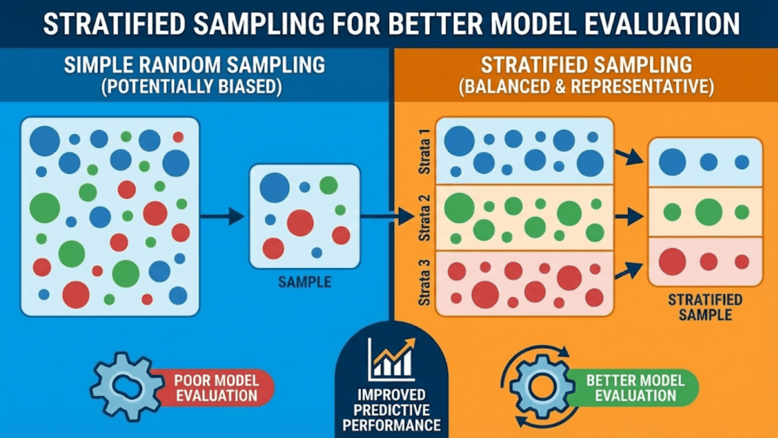
Stratified sampling is a data partitioning technique that ensures each subset (training set, validation set, test set, or cross-validation fold) contains approximately the same proportion of each class or subgroup as the full dataset. Unlike random sampling, which can accidentally create unrepresentative splits — especially with rare classes or small datasets — stratified sampling guarantees that every partition is a faithful miniature of the whole, producing more reliable and reproducible model evaluation metrics.
Introduction
You have a fraud detection dataset: 99,000 legitimate transactions and 1,000 fraudulent ones — a 1% fraud rate. You split it randomly into 80% training and 20% test. With bad luck, your test set ends up with only 150 fraudulent transactions instead of the expected 200. That 25% shortfall in positive examples can make your model’s recall appear much worse than it really is, or cause AUC estimates to vary significantly across different random seeds.
Now imagine running cross-validation with 10 folds. Some folds might receive 80 fraud cases and others only 20 — a 4× difference in minority class representation. The fold with only 20 fraud cases will produce a very different F1 score than the one with 80, making the cross-validation variance artificially high and the final estimate less trustworthy.
These problems disappear with stratified sampling. By ensuring every subset reflects the original class distribution, stratification makes your evaluation metrics more stable, more reproducible, and more representative of real-world performance.
This article covers why stratified sampling matters, how it works mathematically, when to apply it (and when not to), its extension beyond binary classification to continuous targets and multiple grouping variables, and Python implementations for every major use case.
The Problem with Pure Random Sampling
Sampling Variance in Class Proportions
When you randomly sample a fraction of your data, the proportion of each class you get is a random variable. For a dataset with prevalence p (fraction of the positive class) and a sample of size n, the expected proportion of positives is p, but the actual proportion follows a distribution with standard deviation:
For a fraud detection dataset with p=0.01 and a test set of n=2,000:
This means the fraction of fraud cases in your test set will typically vary by ±0.22 percentage points around 1%. With only about 20 fraud cases in a 2,000-sample test set, a swing of even 3–4 cases changes your fraud count by 15–20% — enough to meaningfully shift recall estimates.
Stratification eliminates this variance by fixing the proportion rather than letting it vary randomly.
import numpy as np
import matplotlib.pyplot as plt
from sklearn.model_selection import train_test_split

def demonstrate_random_vs_stratified(n_samples=5000, prevalence=0.05,
                                      test_size=0.20, n_trials=200):
    """
    Compare the stability of class proportions in test sets
    produced by random vs stratified sampling.

    Shows that stratification dramatically reduces variance
    in class representation across splits.
    """
    np.random.seed(42)

    # Generate imbalanced dataset
    n_positive = int(n_samples * prevalence)
    n_negative = n_samples - n_positive
    y = np.array([1] * n_positive + [0] * n_negative)
    X = np.random.randn(n_samples, 5)  # Dummy features

    random_fractions = []
    stratified_fractions = []

    for seed in range(n_trials):
        # Random split
        _, _, _, y_test_rand = train_test_split(
            X, y, test_size=test_size, random_state=seed
        )
        random_fractions.append(y_test_rand.mean())

        # Stratified split
        _, _, _, y_test_strat = train_test_split(
            X, y, test_size=test_size, random_state=seed, stratify=y
        )
        stratified_fractions.append(y_test_strat.mean())

    random_fractions    = np.array(random_fractions)
    stratified_fractions = np.array(stratified_fractions)

    print("=== Random vs Stratified Sampling: Class Proportion Stability ===\n")
    print(f"  Dataset: {n_samples} samples, {prevalence*100:.1f}% positive")
    print(f"  Test size: {test_size*100:.0f}% ({int(n_samples * test_size)} samples)")
    print(f"  Trials: {n_trials}\n")

    print(f"  {'Method':<20} | {'Mean %':>7} | {'Std %':>6} | {'Min %':>6} | {'Max %':>6} | {'Range'}")
    print("  " + "-" * 65)

    for name, fracs in [("Random Sampling", random_fractions),
                         ("Stratified Sampling", stratified_fractions)]:
        print(f"  {name:<20} | {fracs.mean()*100:>7.3f} | {fracs.std()*100:>6.3f} | "
              f"{fracs.min()*100:>6.3f} | {fracs.max()*100:>6.3f} | "
              f"{(fracs.max()-fracs.min())*100:.3f}pp")

    print(f"\n  Stratification reduced std by {random_fractions.std()/stratified_fractions.std():.1f}×")

    # Visualization
    fig, axes = plt.subplots(1, 2, figsize=(14, 5))

    bins = np.linspace(
        min(random_fractions.min(), stratified_fractions.min()),
        max(random_fractions.max(), stratified_fractions.max()),
        30
    )

    for ax, fracs, label, color in [
        (axes[0], random_fractions,    "Random Sampling",    "coral"),
        (axes[1], stratified_fractions, "Stratified Sampling", "steelblue"),
    ]:
        ax.hist(fracs * 100, bins=bins * 100, edgecolor='white', color=color, alpha=0.85)
        ax.axvline(prevalence * 100, color='black', linestyle='--', lw=2,
                   label=f'True prevalence ({prevalence*100:.1f}%)')
        ax.axvline(fracs.mean() * 100, color='darkred', linestyle='-', lw=2,
                   label=f'Mean={fracs.mean()*100:.3f}%')
        ax.set_xlabel("Positive Class % in Test Set", fontsize=11)
        ax.set_ylabel("Frequency (across trials)", fontsize=11)
        ax.set_title(f"{label}\nStd = {fracs.std()*100:.4f}pp",
                     fontsize=12, fontweight='bold')
        ax.legend(fontsize=9)
        ax.grid(True, alpha=0.3)

    plt.suptitle("Distribution of Positive Class % in Test Sets\n"
                 f"({n_trials} trials, {prevalence*100:.1f}% true prevalence)",
                 fontsize=13, fontweight='bold', y=1.02)
    plt.tight_layout()
    plt.savefig("random_vs_stratified_variance.png", dpi=150, bbox_inches='tight')
    plt.show()
    print("Saved: random_vs_stratified_variance.png")

    return random_fractions, stratified_fractions

random_fracs, strat_fracs = demonstrate_random_vs_stratified(
    n_samples=5000, prevalence=0.05, test_size=0.20, n_trials=200
)The Impact on Metric Estimates
The unstable class proportions from random sampling don’t just affect class counts — they directly affect every classification metric. A test set with fewer positive samples produces a different recall, precision, F1, and AUC than one with more. Let’s measure how much:
from sklearn.datasets import make_classification
from sklearn.linear_model import LogisticRegression
from sklearn.model_selection import train_test_split
from sklearn.metrics import f1_score, roc_auc_score
from sklearn.preprocessing import StandardScaler
import numpy as np

def metric_stability_comparison(n_trials=100, prevalence=0.05):
    """
    Compare how stable F1 and AUC estimates are when using
    random vs stratified train-test splits.

    A model trained and evaluated across many random splits
    shows how much metric variance comes from the split alone.
    """
    np.random.seed(42)
    X, y = make_classification(
        n_samples=2000, n_features=15, n_informative=10,
        weights=[1 - prevalence, prevalence], random_state=42
    )

    random_f1s,    random_aucs    = [], []
    stratified_f1s, stratified_aucs = [], []

    for seed in range(n_trials):
        for split_fn, f1_list, auc_list, use_stratify in [
            (False, random_f1s,     random_aucs,     False),
            (True,  stratified_f1s, stratified_aucs, True),
        ]:
            X_tr, X_te, y_tr, y_te = train_test_split(
                X, y, test_size=0.25, random_state=seed,
                stratify=(y if use_stratify else None)
            )

            scaler = StandardScaler()
            X_tr_s = scaler.fit_transform(X_tr)
            X_te_s = scaler.transform(X_te)

            clf = LogisticRegression(class_weight='balanced',
                                     random_state=42, max_iter=500)
            clf.fit(X_tr_s, y_tr)
            y_pred  = clf.predict(X_te_s)
            y_proba = clf.predict_proba(X_te_s)[:, 1]

            f1_list.append(f1_score(y_te, y_pred, zero_division=0))
            auc_list.append(roc_auc_score(y_te, y_proba))

    print(f"\n=== Metric Stability: {n_trials} Trials, {prevalence*100:.0f}% Prevalence ===\n")
    print(f"{'Metric':<8} | {'Method':<22} | {'Mean':>7} | {'Std':>7} | {'Min':>7} | {'Max':>7}")
    print("-" * 65)

    for metric_name, rand_vals, strat_vals in [
        ("F1",  random_f1s,  stratified_f1s),
        ("AUC", random_aucs, stratified_aucs),
    ]:
        for method_name, vals in [("Random", rand_vals), ("Stratified", strat_vals)]:
            vals = np.array(vals)
            print(f"{metric_name:<8} | {method_name:<22} | {vals.mean():>7.4f} | "
                  f"{vals.std():>7.4f} | {vals.min():>7.4f} | {vals.max():>7.4f}")
        print()

    print("Stratified splits consistently produce lower std → more reliable estimates.")

metric_stability_comparison(n_trials=100, prevalence=0.05)How Stratified Sampling Works
The Mechanics
Stratified sampling works by treating each class (or stratum) as a separate population and drawing the appropriate number of samples from each independently.
For a binary dataset with n_pos positive samples and n_neg negative samples, and a desired test fraction of f:
- Draw exactly round(n_pos × f) samples from the positive class
- Draw exactly round(n_neg × f) samples from the negative class
- Combine the two drawn subsets to form the test set
- All remaining samples form the training set
This guarantees that the positive class fraction in both the training and test sets equals (approximately) the original prevalence, regardless of the random seed used for shuffling.
import numpy as np

def manual_stratified_split(X, y, test_size=0.2, random_state=42):
    """
    Implement stratified train-test split from scratch.

    Demonstrates the exact mechanics: sample each class separately,
    then combine to form the final train/test sets.

    Args:
        X:            Feature matrix
        y:            Binary labels (0 or 1)
        test_size:    Fraction of data to use for test
        random_state: Random seed for reproducibility

    Returns:
        X_train, X_test, y_train, y_test
    """
    rng = np.random.RandomState(random_state)
    y   = np.array(y)

    classes      = np.unique(y)
    train_indices = []
    test_indices  = []

    for cls in classes:
        cls_indices = np.where(y == cls)[0]
        rng.shuffle(cls_indices)

        n_test_cls  = max(1, round(len(cls_indices) * test_size))
        n_train_cls = len(cls_indices) - n_test_cls

        test_indices.extend(cls_indices[:n_test_cls])
        train_indices.extend(cls_indices[n_test_cls:])

        print(f"  Class {cls}: {len(cls_indices)} total → "
              f"{n_train_cls} train + {n_test_cls} test")

    train_indices = np.array(train_indices)
    test_indices  = np.array(test_indices)

    return (X[train_indices], X[test_indices],
            y[train_indices], y[test_indices])


# Demonstrate on imbalanced dataset
np.random.seed(42)
n = 1000
y_demo = np.array([1]*50 + [0]*950)   # 5% positive
X_demo = np.random.randn(n, 5)
np.random.shuffle(y_demo)

print("=== Manual Stratified Split ===\n")
print(f"  Full dataset: {n} samples, {y_demo.mean()*100:.1f}% positive\n")
X_tr_m, X_te_m, y_tr_m, y_te_m = manual_stratified_split(X_demo, y_demo, test_size=0.2)

print(f"\n  Results:")
print(f"  Training:   {len(y_tr_m)} samples, {y_tr_m.mean()*100:.2f}% positive")
print(f"  Test:       {len(y_te_m)} samples, {y_te_m.mean()*100:.2f}% positive")
print(f"  Original:   {n} samples, {y_demo.mean()*100:.2f}% positive")
print(f"\n ✓ All three sets have ~5% positive class (stratification preserved)")Multi-Class Stratification
Stratification extends naturally to multi-class problems — each class is sampled separately.
from sklearn.model_selection import train_test_split
import numpy as np

# Multi-class example: 4 classes with very different frequencies
np.random.seed(42)
n = 2000
# Class distribution: 60%, 25%, 10%, 5%
y_multi = np.array(
    [0] * 1200 + [1] * 500 + [2] * 200 + [3] * 100
)
X_multi = np.random.randn(n, 10)

print("=== Multi-Class Stratified Sampling ===\n")
print(f"  Original class distribution:")
for cls in range(4):
    count = (y_multi == cls).sum()
    print(f"    Class {cls}: {count:4d} samples ({count/n*100:5.1f}%)")

X_tr_mc, X_te_mc, y_tr_mc, y_te_mc = train_test_split(
    X_multi, y_multi, test_size=0.20, random_state=42, stratify=y_multi
)

print(f"\n  {'Class':>6} | {'Full %':>8} | {'Train %':>9} | {'Test %':>8} | Match?")
print("  " + "-" * 45)
for cls in range(4):
    full_pct  = (y_multi == cls).mean() * 100
    train_pct = (y_tr_mc == cls).mean() * 100
    test_pct  = (y_te_mc == cls).mean() * 100
    match = "✓" if abs(test_pct - full_pct) < 0.5 else "⚠"
print(f" {cls:>6} | {full_pct:>8.2f} | {train_pct:>9.2f} | {test_pct:>8.2f} | {match}")Stratification for Continuous Targets: Regression
Stratified sampling is typically discussed for classification, but the need for representative splits applies equally to regression. When the target distribution is skewed or multimodal, random splits may place most high-value or low-value examples in one partition.
The solution: bin the continuous target into quantile groups and stratify on those bins.
import numpy as np
import pandas as pd
from sklearn.model_selection import train_test_split
import matplotlib.pyplot as plt

def stratified_regression_split(X, y, test_size=0.20, n_bins=10, random_state=42):
    """
    Perform stratified train-test split for regression by
    binning the continuous target into quantile groups.

    Args:
        X:            Feature matrix
        y:            Continuous target variable
        test_size:    Fraction for test set
        n_bins:       Number of quantile bins for stratification
        random_state: Random seed

    Returns:
        X_train, X_test, y_train, y_test
    """
    # Bin target into quantile groups
    y_binned = pd.qcut(y, q=n_bins, labels=False, duplicates='drop')

    X_train, X_test, y_train, y_test = train_test_split(
        X, y, test_size=test_size, random_state=random_state,
        stratify=y_binned
    )
    return X_train, X_test, y_train, y_test


def compare_regression_splits(n_samples=2000, test_size=0.20, n_trials=100):
    """
    Compare target distribution representativeness in test sets
    from random vs stratified regression splits.
    """
    np.random.seed(42)

    # Create skewed target: log-normal (like house prices, income, etc.)
    y_reg = np.exp(np.random.normal(0, 1.5, n_samples))
    X_reg = np.random.randn(n_samples, 5)

    rand_means,  strat_means  = [], []
    rand_stds,   strat_stds   = [], []
    rand_p90s,   strat_p90s   = [], []

    for seed in range(n_trials):
        # Random split
        _, _, _, y_te_rand = train_test_split(
            X_reg, y_reg, test_size=test_size, random_state=seed
        )
        rand_means.append(y_te_rand.mean())
        rand_stds.append(y_te_rand.std())
        rand_p90s.append(np.percentile(y_te_rand, 90))

        # Stratified split
        _, _, _, y_te_strat = stratified_regression_split(
            X_reg, y_reg, test_size=test_size, random_state=seed
        )
        strat_means.append(y_te_strat.mean())
        strat_stds.append(y_te_strat.std())
        strat_p90s.append(np.percentile(y_te_strat, 90))

    print("=== Regression Splits: Target Distribution Stability ===\n")
    print(f"  True target: mean={y_reg.mean():.3f}, std={y_reg.std():.3f}, "
          f"90th pct={np.percentile(y_reg, 90):.3f}\n")

    print(f"  {'Statistic':<15} | {'Random Std':>12} | {'Stratified Std':>15} | {'Improvement'}")
    print("  " + "-" * 60)

    for stat_name, rand_vals, strat_vals in [
        ("Mean",   rand_means, strat_means),
        ("Std",    rand_stds,  strat_stds),
        ("90th %", rand_p90s,  strat_p90s),
    ]:
        r_std = np.std(rand_vals)
        s_std = np.std(strat_vals)
        improvement = r_std / s_std if s_std > 0 else float('inf')
        print(f"  {stat_name:<15} | {r_std:>12.4f} | {s_std:>15.4f} | "
              f"{improvement:.1f}× lower std")

compare_regression_splits()Stratification Across Multiple Variables
Sometimes you need to ensure representativeness across multiple dimensions simultaneously — class label AND age group AND geographic region, for example. Multilabel stratification (or joint stratification) handles this case.
import numpy as np
import pandas as pd
from sklearn.model_selection import train_test_split

def create_joint_stratum(df, stratify_cols):
    """
    Create a combined stratification key from multiple columns.

    Encodes combinations of values across all stratification columns
    into a single integer that can be used with stratify= parameter.

    Args:
        df:             Pandas DataFrame
        stratify_cols:  List of column names to stratify jointly

    Returns:
        Array of integer stratum IDs, one per row
    """
    # Create string representation of each unique combination
    combined = df[stratify_cols].astype(str).apply(lambda row: '_'.join(row), axis=1)

    # Count samples per stratum — strata with very few samples may cause issues
    stratum_counts = combined.value_counts()
    rare_strata    = stratum_counts[stratum_counts < 5].index

    if len(rare_strata) > 0:
        print(f"  ⚠ Warning: {len(rare_strata)} rare strata with <5 samples.")
        print(f"  These may cause issues with stratification. Consider grouping.")

    # Encode as integers
    unique_strata = combined.unique()
    stratum_map   = {s: i for i, s in enumerate(unique_strata)}
    return combined.map(stratum_map).values


# Example: Clinical trial with disease severity + gender + age group
np.random.seed(42)
n = 800

df_clinical = pd.DataFrame({
    'label':       np.random.choice([0, 1], size=n, p=[0.75, 0.25]),
    'severity':    np.random.choice(['mild', 'moderate', 'severe'], size=n, p=[0.5, 0.35, 0.15]),
    'sex':         np.random.choice(['M', 'F'], size=n, p=[0.48, 0.52]),
    'age_group':   np.random.choice(['18-40', '41-60', '61+'], size=n, p=[0.35, 0.40, 0.25]),
})
X_clinical = np.random.randn(n, 10)

print("=== Multilabel Stratification ===\n")
print("  Stratifying jointly on: label + severity + sex + age_group\n")

# Create joint stratum key
stratum_key = create_joint_stratum(df_clinical, ['label', 'severity', 'sex', 'age_group'])

print(f"  Unique strata: {len(np.unique(stratum_key))}")
print(f"  (2 labels × 3 severities × 2 sexes × 3 age groups = {2*3*2*3} max combinations)\n")

X_tr_cl, X_te_cl, df_tr, df_te, s_tr, s_te = train_test_split(
    X_clinical, df_clinical, stratum_key,
    test_size=0.20, random_state=42, stratify=stratum_key
)

# Verify preservation of each variable's distribution
print(f"  {'Variable':<12} | {'Category':<12} | {'Full %':>8} | {'Train %':>9} | {'Test %':>8}")
print("  " + "-" * 55)

for col in ['label', 'severity', 'sex', 'age_group']:
    for val in sorted(df_clinical[col].unique()):
        full_pct  = (df_clinical[col] == val).mean() * 100
        train_pct = (df_tr[col] == val).mean() * 100
        test_pct  = (df_te[col] == val).mean() * 100
        print(f"  {col:<12} | {str(val):<12} | {full_pct:>8.1f} | {train_pct:>9.1f} | {test_pct:>8.1f}")
    print()
Stratified Sampling in Cross-Validation
Stratification in cross-validation is even more important than in a single train-test split because the validation sets are smaller (1/K of the development data), making them more susceptible to class imbalance.
from sklearn.model_selection import (
    KFold, StratifiedKFold, RepeatedStratifiedKFold,
    cross_val_score, cross_validate
)
from sklearn.ensemble import GradientBoostingClassifier, RandomForestClassifier
from sklearn.linear_model import LogisticRegression
from sklearn.pipeline import Pipeline
from sklearn.preprocessing import StandardScaler
from sklearn.metrics import make_scorer, f1_score, roc_auc_score
from sklearn.datasets import make_classification
import numpy as np

def compare_cv_stratification(X, y, k=5, n_repeats=10, random_state=42):
    """
    Compare KFold vs StratifiedKFold cross-validation in terms of:
    1. Class distribution stability across folds
    2. Metric estimate stability
    3. Practical differences in reported performance
    """
    np.random.seed(random_state)

    model = Pipeline([
        ('scaler', StandardScaler()),
        ('clf', LogisticRegression(class_weight='balanced', random_state=42, max_iter=1000))
    ])

    auc_scorer = make_scorer(roc_auc_score, needs_proba=True)
    f1_scorer  = make_scorer(f1_score, zero_division=0)

    results = {}
    for cv_class, cv_name in [
        (KFold(n_splits=k, shuffle=True, random_state=random_state),
         f"{k}-Fold (no stratification)"),
        (StratifiedKFold(n_splits=k, shuffle=True, random_state=random_state),
         f"Stratified {k}-Fold"),
        (RepeatedStratifiedKFold(n_splits=k, n_repeats=n_repeats, random_state=random_state),
         f"Repeated Stratified {k}-Fold ({n_repeats}×)"),
    ]:
        cv_result = cross_validate(
            model, X, y, cv=cv_class,
            scoring={'auc': auc_scorer, 'f1': f1_scorer},
            return_train_score=False, n_jobs=-1
        )
        results[cv_name] = cv_result

    print(f"\n=== CV Stratification Comparison ===")
    print(f"  Dataset: {len(y)} samples, {y.mean()*100:.1f}% positive\n")
    print(f"  {'CV Strategy':<40} | {'AUC Mean':>9} | {'AUC Std':>8} | {'F1 Mean':>8} | {'F1 Std':>7}")
    print("  " + "-" * 80)

    for name, result in results.items():
        auc_mean = result['test_auc'].mean()
        auc_std  = result['test_auc'].std()
        f1_mean  = result['test_f1'].mean()
        f1_std   = result['test_f1'].std()
        print(f"  {name:<40} | {auc_mean:>9.4f} | {auc_std:>8.4f} | {f1_mean:>8.4f} | {f1_std:>7.4f}")

    return results

# Highly imbalanced dataset
np.random.seed(42)
X_cv, y_cv = make_classification(
    n_samples=1000, n_features=15, n_informative=10,
    weights=[0.92, 0.08], random_state=42  # Only 8% positive
)

cv_comparison = compare_cv_stratification(X_cv, y_cv, k=5, n_repeats=10)The Fold-Level Class Distribution Check
Before running cross-validation, always verify that each fold has sufficient minority class representation:
from sklearn.model_selection import StratifiedKFold
import numpy as np

def audit_cv_fold_distributions(X, y, cv, min_positive_per_fold=5):
    """
    Audit class distributions across all CV folds.

    Args:
        X, y:                    Features and labels
        cv:                      Cross-validator object
        min_positive_per_fold:   Minimum acceptable positive count per fold

    Returns:
        Audit report with pass/fail per fold
    """
    print(f"=== CV Fold Class Distribution Audit ===\n")
    print(f"  Overall: {len(y)} samples, {y.sum()} positive ({y.mean()*100:.1f}%)")
    print(f"  Minimum acceptable positives per fold: {min_positive_per_fold}\n")

    fold_stats = []
    all_pass = True

    print(f"  {'Fold':>6} | {'Train N':>8} | {'Train pos%':>11} | "
          f"{'Test N':>7} | {'Test pos%':>10} | {'Test #pos':>9} | Status")
    print("  " + "-" * 75)

    for fold_i, (train_idx, test_idx) in enumerate(cv.split(X, y), 1):
        y_tr_fold = y[train_idx]
        y_te_fold = y[test_idx]

        n_pos_test = y_te_fold.sum()
        status = "✓ OK" if n_pos_test >= min_positive_per_fold else "⚠ LOW"
        if n_pos_test < min_positive_per_fold:
            all_pass = False

        print(f"  {fold_i:>6} | {len(y_tr_fold):>8} | {y_tr_fold.mean()*100:>10.2f}% | "
              f"{len(y_te_fold):>7} | {y_te_fold.mean()*100:>9.2f}% | "
              f"{n_pos_test:>9} | {status}")

        fold_stats.append(n_pos_test)

    print(f"\n  Positive count range: {min(fold_stats)} – {max(fold_stats)}")
    print(f"  Overall audit: {'✓ PASS' if all_pass else '⚠ FAIL — consider using fewer folds or oversampling'}")

    return fold_stats


# Test on severely imbalanced data
np.random.seed(42)
X_aud, y_aud = make_classification(
    n_samples=500, n_features=10,
    weights=[0.97, 0.03],  # Only 3% positive → 15 positive samples total
    random_state=42
)

print("Test 1: Stratified K-Fold (should pass if k is reasonable)\n")
skf_aud = StratifiedKFold(n_splits=5, shuffle=True, random_state=42)
audit_cv_fold_distributions(X_aud, y_aud, skf_aud, min_positive_per_fold=3)Practical Applications of Stratified Sampling
Application 1: Medical Diagnosis Dataset
from sklearn.datasets import load_breast_cancer
from sklearn.model_selection import train_test_split, StratifiedKFold, cross_val_score
from sklearn.ensemble import RandomForestClassifier
from sklearn.metrics import make_scorer, f1_score, recall_score
import numpy as np

# Load breast cancer dataset (37% malignant — moderately imbalanced)
data = load_breast_cancer()
X_bc, y_bc = data.data, data.target

print("=== Breast Cancer Detection: Stratified Evaluation ===\n")
print(f"  Dataset: {len(y_bc)} samples")
print(f"  Class 0 (malignant): {(y_bc==0).sum()} ({(y_bc==0).mean()*100:.1f}%)")
print(f"  Class 1 (benign):    {(y_bc==1).sum()} ({(y_bc==1).mean()*100:.1f}%)\n")

# Always stratify the initial holdout split
X_bc_dev, X_bc_hold, y_bc_dev, y_bc_hold = train_test_split(
    X_bc, y_bc, test_size=0.20, random_state=42, stratify=y_bc
)

print(f"  After stratified split:")
print(f"  Dev   ({len(y_bc_dev)} samples): {y_bc_dev.mean()*100:.1f}% benign")
print(f"  Hold  ({len(y_bc_hold)} samples): {y_bc_hold.mean()*100:.1f}% benign")

# Stratified cross-validation on dev set
# Medical context: recall for malignant (class 0) is critical
recall_scorer = make_scorer(recall_score, pos_label=0, zero_division=0)

skf_bc = StratifiedKFold(n_splits=5, shuffle=True, random_state=42)
rf_bc  = RandomForestClassifier(100, random_state=42, n_jobs=-1)

cv_recall = cross_val_score(rf_bc, X_bc_dev, y_bc_dev, cv=skf_bc,
                             scoring=recall_scorer)
cv_f1     = cross_val_score(rf_bc, X_bc_dev, y_bc_dev, cv=skf_bc,
                             scoring='f1')

print(f"\n  Stratified 5-Fold CV Results (Dev Set):")
print(f"  Recall (malignant): {cv_recall.mean():.4f} ± {cv_recall.std():.4f}")
print(f" F1 Score: {cv_f1.mean():.4f} ± {cv_f1.std():.4f}")Application 2: Extremely Imbalanced Fraud Detection
When positive class prevalence drops below 1%, standard stratification may still leave some folds with very few positives. The solution is to combine stratification with oversampling or to reduce the number of folds.
from sklearn.datasets import make_classification
from sklearn.model_selection import StratifiedKFold, cross_val_score
from sklearn.ensemble import GradientBoostingClassifier
from sklearn.metrics import make_scorer, average_precision_score
import numpy as np

# Very imbalanced dataset: 0.5% fraud rate
np.random.seed(42)
X_fraud, y_fraud = make_classification(
    n_samples=10000,
    n_features=20,
    n_informative=12,
    weights=[0.995, 0.005],  # 0.5% fraud
    random_state=42
)

n_fraud = y_fraud.sum()
print(f"=== Fraud Detection: {y_fraud.mean()*100:.2f}% Prevalence ===\n")
print(f"  Total transactions: {len(y_fraud):,}")
print(f"  Fraudulent: {n_fraud} ({y_fraud.mean()*100:.2f}%)")

# Choose k such that each fold has at least 5 fraudulent samples
max_k = n_fraud // 5
safe_k = min(10, max_k)
print(f"\n  Maximum safe K for ≥5 fraud per fold: {max_k}")
print(f"  Using K = {safe_k}")

ap_scorer = make_scorer(average_precision_score, needs_proba=True)
gbm_fraud = GradientBoostingClassifier(100, random_state=42)

skf_fraud = StratifiedKFold(n_splits=safe_k, shuffle=True, random_state=42)
ap_scores = cross_val_score(gbm_fraud, X_fraud, y_fraud,
                             cv=skf_fraud, scoring=ap_scorer, n_jobs=-1)

print(f"\n  {safe_k}-Fold Stratified CV Average Precision:")
print(f"  {ap_scores.mean():.4f} ± {ap_scores.std():.4f}")
print(f" (AP = area under precision-recall curve; better than AUC for extreme imbalance)")Stratification and the Holdout Test Set
One principle that applies universally: the holdout test set must be stratified at the moment it is created, before any model development begins. Failing to stratify the initial split means your test set may be unrepresentative, and every conclusion you draw about final model performance will be slightly (or significantly) wrong.
from sklearn.model_selection import train_test_split
from sklearn.ensemble import RandomForestClassifier, GradientBoostingClassifier
from sklearn.linear_model import LogisticRegression
from sklearn.pipeline import Pipeline
from sklearn.preprocessing import StandardScaler
from sklearn.metrics import roc_auc_score, f1_score, average_precision_score
from sklearn.datasets import make_classification
import numpy as np

def production_stratified_evaluation_pipeline(X, y,
                                               holdout_size=0.15,
                                               dev_cv_splits=5,
                                               dev_cv_repeats=3,
                                               random_state=42):
    """
    Complete production-quality stratified evaluation pipeline.

    Implements all best practices:
    1. Stratified holdout split first
    2. Stratified repeated cross-validation on dev set
    3. Model selection based on CV AUC
    4. Final evaluation on holdout (once, at the end)

    Args:
        X, y:             Features and labels
        holdout_size:     Fraction for final test set
        dev_cv_splits:    Number of CV folds on dev set
        dev_cv_repeats:   Number of CV repetitions
        random_state:     Random seed
    """
    from sklearn.model_selection import RepeatedStratifiedKFold, cross_validate
    from sklearn.metrics import make_scorer

    print(f"{'='*60}")
    print(f"  STRATIFIED EVALUATION PIPELINE")
    print(f"{'='*60}")
    print(f"\n  Dataset: {len(y):,} samples, {y.mean()*100:.2f}% positive\n")

    # ── Step 1: Stratified holdout split ──────────────────────
    X_dev, X_hold, y_dev, y_hold = train_test_split(
        X, y, test_size=holdout_size, random_state=random_state, stratify=y
    )

    print(f"  Step 1: Stratified Holdout Split")
    print(f"    Dev set:  {len(y_dev):,} samples ({y_dev.mean()*100:.2f}% pos)")
    print(f"    Holdout:  {len(y_hold):,} samples ({y_hold.mean()*100:.2f}% pos)")

    # ── Step 2: CV model comparison ───────────────────────────
    models_prod = {
        "Logistic Regression": Pipeline([
            ('scaler', StandardScaler()),
            ('clf', LogisticRegression(class_weight='balanced',
                                        random_state=random_state, max_iter=1000))
        ]),
        "Random Forest": RandomForestClassifier(
            200, class_weight='balanced', random_state=random_state, n_jobs=-1
        ),
        "Gradient Boosting": GradientBoostingClassifier(
            200, random_state=random_state
        ),
    }

    rskf = RepeatedStratifiedKFold(
        n_splits=dev_cv_splits, n_repeats=dev_cv_repeats, random_state=random_state
    )

    auc_scorer = make_scorer(roc_auc_score, needs_proba=True)
    ap_scorer  = make_scorer(average_precision_score, needs_proba=True)

    print(f"\n  Step 2: Stratified CV on Dev Set "
          f"({dev_cv_splits}-Fold × {dev_cv_repeats} repeats)")
    print(f"\n  {'Model':<25} | {'AUC':>8} | {'±':>7} | {'AP':>8} | {'±':>7}")
    print("  " + "-" * 58)

    best_auc = -1
    best_model_name = None
    cv_summary = {}

    for name, model in models_prod.items():
        cv_res = cross_validate(
            model, X_dev, y_dev, cv=rskf,
            scoring={'auc': auc_scorer, 'ap': ap_scorer},
            n_jobs=-1
        )

        auc_m = cv_res['test_auc'].mean()
        auc_s = cv_res['test_auc'].std()
        ap_m  = cv_res['test_ap'].mean()
        ap_s  = cv_res['test_ap'].std()

        cv_summary[name] = {'auc': auc_m, 'auc_std': auc_s,
                             'ap': ap_m, 'ap_std': ap_s}

        flag = " ← best" if auc_m > best_auc else ""
        print(f"  {name:<25} | {auc_m:>8.4f} | {auc_s:>7.4f} | {ap_m:>8.4f} | {ap_s:>7.4f}{flag}")

        if auc_m > best_auc:
            best_auc = auc_m
            best_model_name = name

    # ── Step 3: Final evaluation on holdout ───────────────────
    print(f"\n  Step 3: Final Holdout Evaluation")
    print(f"  Best model (by CV AUC): {best_model_name}")

    best_model = models_prod[best_model_name]
    best_model.fit(X_dev, y_dev)

    y_hold_proba = best_model.predict_proba(X_hold)[:, 1]
    y_hold_pred  = (y_hold_proba >= 0.5).astype(int)

    hold_auc = roc_auc_score(y_hold, y_hold_proba)
    hold_ap  = average_precision_score(y_hold, y_hold_proba)
    hold_f1  = f1_score(y_hold, y_hold_pred, zero_division=0)

    cv_auc = cv_summary[best_model_name]['auc']

    print(f"\n  {'Metric':<15} | {'CV Estimate':>12} | {'Holdout':>8} | {'Gap'}")
    print("  " + "-" * 50)
    print(f"  {'AUC-ROC':<15} | {cv_auc:>12.4f} | {hold_auc:>8.4f} | {hold_auc - cv_auc:+.4f}")
    print(f"  {'Avg Precision':<15} | {cv_summary[best_model_name]['ap']:>12.4f} | {hold_ap:>8.4f} | "
          f"{hold_ap - cv_summary[best_model_name]['ap']:+.4f}")

    optimism = abs(cv_auc - hold_auc)
    print(f"\n  CV optimism: {optimism:.4f} "
          f"({'acceptable (<0.02)' if optimism < 0.02 else 'notable — check for leakage'})")


# Run the complete pipeline
np.random.seed(42)
X_prod, y_prod = make_classification(
    n_samples=3000, n_features=20, n_informative=14,
    weights=[0.88, 0.12], random_state=42
)

production_stratified_evaluation_pipeline(X_prod, y_prod)The Statistics Behind Stratification: Why It Works
Understanding the mathematical foundation of stratified sampling clarifies both why it works and when it provides the most benefit.
Variance Reduction in Proportion Estimates
Consider estimating the population mean of some statistic (say, the positive class rate) using a sample. In simple random sampling, the variance of the sample mean is:
where S² is the population variance and n is the sample size. In stratified sampling where we sample proportionally from H strata, the variance becomes:
where W_h is the weight of stratum h (its proportion in the population) and S_h² is the variance within stratum h. The key insight: stratified sampling replaces the total population variance with a weighted sum of within-stratum variances. When strata are internally homogeneous (little variation within each class), this sum is much smaller than the total variance, producing a much lower-variance estimator.
For classification, the strata are the class labels themselves. Within the positive class, every sample is positive (variance = 0 for the class indicator). The only variance comes from feature variation, not from class membership. This is exactly why stratified sampling on class labels is so effective — it eliminates the between-class component of variance from your split entirely.
Design Effect
The design effect (DEFF) quantifies how much more (or less) efficient a sampling design is compared to simple random sampling:
A DEFF < 1 means the stratified design is more efficient than random sampling — you get the same precision with fewer samples, or more precision with the same number. For proportional stratified sampling on class labels, the DEFF on class proportion estimates is essentially 0 (we know the class proportion exactly after stratification). This is the theoretical basis for the dramatic variance reduction you observed in the simulation above.
import numpy as np
from scipy import stats

def theoretical_variance_analysis(n_total, prevalence, test_fraction):
    """
    Compute theoretical variance of positive class proportion estimate
    under random vs stratified sampling.

    Args:
        n_total:        Total dataset size
        prevalence:     True positive class fraction
        test_fraction:  Fraction of data in test set

    Returns:
        Dictionary with theoretical standard deviations
    """
    n_test = int(n_total * test_fraction)
    n_pos  = int(n_total * prevalence)
    n_neg  = n_total - n_pos

    # ── Random sampling (binomial model) ──────────────────────
    # Under random sampling, the number of positives in a test set
    # of size n_test follows a hypergeometric distribution
    # (without replacement from finite population)
    # Variance of hypergeometric proportion:
    var_random = (prevalence * (1 - prevalence) / n_test) * (
        (n_total - n_test) / (n_total - 1)  # Finite population correction
    )
    std_random = np.sqrt(var_random)

    # ── Stratified sampling (fixed counts per class) ──────────
    # After stratification, the exact number of positives in the test set
    # is deterministic: round(n_pos * test_fraction)
    # Variance of the proportion estimate is essentially 0 for the
    # class proportion itself (it's exactly fixed by construction)
    # Remaining variance only comes from which specific samples are chosen
    n_pos_test  = round(n_pos * test_fraction)
    n_neg_test  = round(n_neg * test_fraction)

    # Variance due to sampling within each class (which specific positives chosen)
    # This is much smaller: now we're sampling from within-class feature distributions
    var_stratified = 0  # For the class proportion itself — it's fixed
    std_stratified = 0

    print(f"=== Theoretical Variance Analysis ===\n")
    print(f"  Dataset: {n_total:,} samples, {prevalence*100:.1f}% positive")
    print(f"  Test set: {test_fraction*100:.0f}% ({n_test:,} samples)")
    print(f"  Expected positives in test set: {n_pos_test}")

    print(f"\n  Under random sampling:")
    print(f"    Std of positive fraction in test set: {std_random:.5f}")
    print(f"    95% CI: [{(prevalence - 2*std_random)*100:.3f}%, {(prevalence + 2*std_random)*100:.3f}%]")
    print(f"    → Test set can have {n_test*(prevalence - 2*std_random):.1f}–{n_test*(prevalence + 2*std_random):.1f} positives")

    print(f"\n  Under stratified sampling:")
    print(f"    Positive count in test set: exactly {n_pos_test} (fixed by construction)")
    print(f"    Std of positive fraction: 0 (deterministic)")
    print(f"    → Test set always has exactly {n_pos_test} positives")

    print(f"\n  Variance reduction factor: ∞ (from non-zero to zero)")
    print(f"  Any sampling variance in metric estimates comes only from")
    print(f"  which specific positive/negative samples were selected,")
    print(f"  not from how many of each class were included.")

theoretical_variance_analysis(n_total=10000, prevalence=0.05, test_fraction=0.20)Proportional vs Optimal Allocation
In survey statistics, proportional allocation places each stratum in the sample proportional to its size in the population — which is exactly what scikit-learn’s stratify= does. However, there is also optimal (Neyman) allocation, which assigns more samples from strata with higher variance:
For model evaluation, proportional allocation is almost always the right choice — you want your test set to reflect real-world class distributions. Optimal allocation would be relevant only if you were trying to estimate a population parameter with minimum variance, not if you wanted a representative model evaluation.
Interaction Between Stratification and Data Augmentation
A subtle issue arises when using data augmentation or oversampling (like SMOTE) alongside cross-validation: augmentation must happen inside the cross-validation loop, not before it. If you oversample the full dataset and then split it, synthetic samples from the minority class will appear in both training and validation sets, constituting data leakage.
import numpy as np
from sklearn.datasets import make_classification
from sklearn.model_selection import StratifiedKFold
from sklearn.linear_model import LogisticRegression
from sklearn.preprocessing import StandardScaler
from sklearn.metrics import roc_auc_score

def cv_with_proper_oversampling(X, y, n_splits=5, random_state=42):
    """
    Demonstrate the correct way to combine SMOTE with stratified CV:
    oversample inside each fold, never before splitting.

    Compares:
    1. Correct: SMOTE inside CV loop (no leakage)
    2. Incorrect: SMOTE before CV split (leakage)

    Note: Requires imbalanced-learn (pip install imbalanced-learn)
    If not available, demonstrates the concept with random oversampling.
    """
    try:
        from imblearn.over_sampling import SMOTE
        use_smote = True
    except ImportError:
        use_smote = False
        print("  (imbalanced-learn not available — using random oversampling)")

    skf = StratifiedKFold(n_splits=n_splits, shuffle=True, random_state=random_state)

    # ── Correct: Oversample inside each fold ──────────────────
    correct_aucs = []
    for fold_i, (train_idx, test_idx) in enumerate(skf.split(X, y)):
        X_tr, X_te = X[train_idx], X[test_idx]
        y_tr, y_te = y[train_idx], y[test_idx]

        # Scale before oversampling
        scaler = StandardScaler()
        X_tr_s = scaler.fit_transform(X_tr)
        X_te_s = scaler.transform(X_te)

        # Oversample ONLY the training fold
        if use_smote:
            from imblearn.over_sampling import SMOTE
            sm = SMOTE(random_state=random_state)
            X_tr_resampled, y_tr_resampled = sm.fit_resample(X_tr_s, y_tr)
        else:
            # Random oversampling of minority class
            pos_idx = np.where(y_tr == 1)[0]
            n_neg   = (y_tr == 0).sum()
            oversample_idx = np.random.choice(pos_idx, size=n_neg, replace=True)
            all_idx = np.concatenate([np.where(y_tr == 0)[0], oversample_idx])
            X_tr_resampled = X_tr_s[all_idx]
            y_tr_resampled = y_tr[all_idx]

        # Train and evaluate
        clf = LogisticRegression(random_state=random_state, max_iter=1000)
        clf.fit(X_tr_resampled, y_tr_resampled)
        y_proba = clf.predict_proba(X_te_s)[:, 1]
        correct_aucs.append(roc_auc_score(y_te, y_proba))

    # ── Incorrect: Oversample before splitting (leakage!) ─────
    if use_smote:
        from imblearn.over_sampling import SMOTE
        sm_pre = SMOTE(random_state=random_state)
        X_oversampled, y_oversampled = sm_pre.fit_resample(X, y)
    else:
        pos_idx = np.where(y == 1)[0]
        n_neg_all = (y == 0).sum()
        oversample_idx = np.random.choice(pos_idx, size=n_neg_all, replace=True)
        all_idx_pre = np.concatenate([np.where(y == 0)[0], oversample_idx])
        np.random.shuffle(all_idx_pre)
        X_oversampled = X[all_idx_pre]
        y_oversampled = y[all_idx_pre]

    leaky_aucs = []
    # Note: no stratification needed after SMOTE since classes are balanced
    from sklearn.model_selection import KFold
    kf_leaky = KFold(n_splits=n_splits, shuffle=True, random_state=random_state)

    for fold_i, (train_idx, test_idx) in enumerate(kf_leaky.split(X_oversampled)):
        X_tr_l, X_te_l = X_oversampled[train_idx], X_oversampled[test_idx]
        y_tr_l, y_te_l = y_oversampled[train_idx], y_oversampled[test_idx]

        scaler_l = StandardScaler()
        X_tr_sl = scaler_l.fit_transform(X_tr_l)
        X_te_sl = scaler_l.transform(X_te_l)

        clf_l = LogisticRegression(random_state=random_state, max_iter=1000)
        clf_l.fit(X_tr_sl, y_tr_l)
        y_proba_l = clf_l.predict_proba(X_te_sl)[:, 1]
        leaky_aucs.append(roc_auc_score(y_te_l, y_proba_l))

    print(f"\n=== Oversampling + Stratified CV: Correct vs Incorrect ===\n")
    print(f"  ✓ Correct (SMOTE inside each fold): AUC = {np.mean(correct_aucs):.4f} ± {np.std(correct_aucs):.4f}")
    print(f"  ✗ Incorrect (SMOTE before split):   AUC = {np.mean(leaky_aucs):.4f} ± {np.std(leaky_aucs):.4f}")
    print(f"\n  Leakage inflation: +{np.mean(leaky_aucs) - np.mean(correct_aucs):.4f}")
    print(f"  (Synthetic samples in test set make performance look better than it is)")
    print(f"\n  Always apply oversampling inside the CV loop — never before splitting!")


# Run the demonstration
np.random.seed(42)
X_smote, y_smote = make_classification(
    n_samples=1000, n_features=15, n_informative=8,
    weights=[0.90, 0.10], random_state=42
)

cv_with_proper_oversampling(X_smote, y_smote, n_splits=5)The correct approach uses scikit-learn’s Pipeline combined with imblearn‘s Pipeline (which supports oversampling steps), or manually applies oversampling inside each fold as shown above. The imblearn.pipeline.Pipeline class handles this automatically and is the recommended production approach.
When Not to Stratify
Stratification is almost always beneficial, but a few situations call for caution:
Very small minority class: If you have fewer than K samples in the minority class, stratified K-Fold will fail (it cannot guarantee even one positive sample per fold). In this case, reduce K, use LOO-CV, or handle the class imbalance problem before splitting.
Time series data: Stratification shuffles data randomly, destroying temporal order. For time series, use TimeSeriesSplit even if the series has imbalanced labels.
Grouped data where group matters more than class: If preserving group integrity (patients, users) matters more than class balance, use GroupKFold. You can combine grouping with stratification using StratifiedGroupKFold in scikit-learn ≥ 1.1.
Regression without distributional concerns: If your target variable is approximately normally distributed and your dataset is large enough, random splitting will naturally produce representative test sets. Stratification adds minimal value in this case.
from sklearn.model_selection import StratifiedGroupKFold
import numpy as np

# Combined group + stratification: patients with disease labels
np.random.seed(42)
n = 500
patient_ids = np.repeat(np.arange(100), 5)    # 100 patients, 5 measurements each
labels      = np.random.binomial(1, 0.25, 500) # 25% positive

print("=== StratifiedGroupKFold: Group Integrity + Class Balance ===\n")
print(f"  Dataset: {n} measurements, {len(np.unique(patient_ids))} patients")
print(f"  Positive rate: {labels.mean()*100:.1f}%\n")

X_sgkf = np.random.randn(n, 10)
sgkf   = StratifiedGroupKFold(n_splits=5)

print(f"  {'Fold':>6} | {'Train Pat.':>12} | {'Test Pat.':>11} | "
      f"{'Train pos%':>11} | {'Test pos%':>10} | Overlap?")
print("  " + "-" * 72)

for fold_i, (tr_idx, te_idx) in enumerate(
        sgkf.split(X_sgkf, labels, groups=patient_ids), 1):

    tr_patients = set(patient_ids[tr_idx])
    te_patients = set(patient_ids[te_idx])
    overlap     = tr_patients & te_patients

    tr_pos_pct = labels[tr_idx].mean() * 100
    te_pos_pct = labels[te_idx].mean() * 100

    status = f"⚠ OVERLAP" if overlap else "✓ Clean"
    print(f"  {fold_i:>6} | {len(tr_patients):>12} | {len(te_patients):>11} | "
f"{tr_pos_pct:>10.1f}% | {te_pos_pct:>9.1f}% | {status}")Summary
Stratified sampling is one of those techniques that seems like a minor implementation detail but has significant effects on the reliability and reproducibility of model evaluation — especially for the imbalanced class distributions that characterize almost every real-world problem of interest.
The core principle is simple: every subset of your data should be a faithful representative sample of the whole. When class distributions vary widely across your train, validation, and test sets, your performance metrics become noisy functions of which specific samples happened to land where — rather than stable measurements of your model’s true capability.
Stratification eliminates this noise source by construction. For binary and multi-class classification, it ensures each subset has approximately the same class proportions as the full dataset. For regression, binning the target into quantiles before stratifying achieves the same goal. For datasets with multiple grouping dimensions — disease severity, age group, geography — joint stratification preserves their joint distributions simultaneously.
The practical rules that emerge from this are straightforward: always stratify your initial holdout split, always use Stratified K-Fold for classification cross-validation, audit your fold class distributions for severely imbalanced datasets, combine stratification with group constraints using StratifiedGroupKFold when samples are not independent, and use quantile-based stratification for regression problems with skewed targets.
These habits pay dividends every time you compare models, tune hyperparameters, or report final results. The stability they introduce into your evaluation process is not a theoretical nicety — it is the difference between reproducible, trustworthy results and conclusions that evaporate when a different random seed is used.