Polynomial regression extends linear regression to model curved, non-linear relationships by adding polynomial terms (x², x³, etc.) as new features. Although the relationship between the input x and output y is curved, the model remains linear in its parameters — it is still linear regression applied to transformed features. For example, a degree-2 polynomial fits ŷ = w₁x + w₂x² + b, capturing a parabola. Higher degrees capture more complex curves but risk overfitting, making degree selection through cross-validation essential.
Introduction: When Data Curves
Not all relationships between variables are straight lines. A drug’s effectiveness increases with dosage up to a point, then plateaus or even decreases. A car’s fuel efficiency improves as speed increases from city to highway, then worsens at very high speeds. Employee productivity grows with experience early in a career, then levels off. Population growth accelerates exponentially, then slows as resources become constrained.
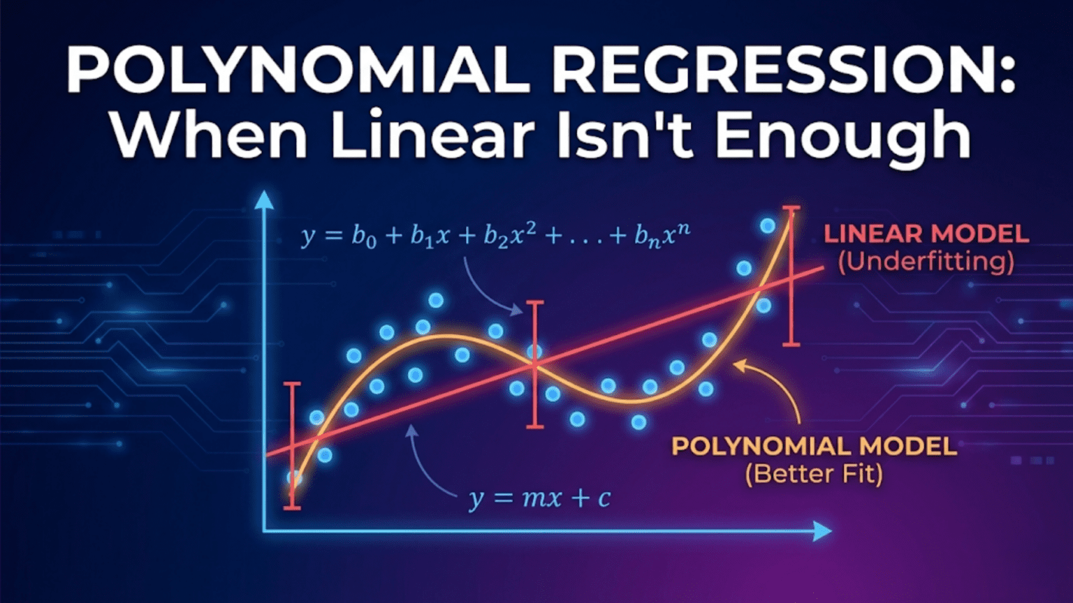
These curved relationships are everywhere in nature, science, business, and human behavior. Simple and multiple linear regression can’t capture them — no matter how many linear features you include, you can only fit planes and hyperplanes to data, not curves and waves.
Polynomial regression solves this problem elegantly. By adding polynomial powers of the original features as new inputs — x becomes x, x², x³, and so on — the model gains the flexibility to follow curves in the data. The mathematical insight is beautiful: even though the relationship between x and y is non-linear, the relationship between the polynomial features and y is still linear. This means all the machinery of linear regression — the cost function, gradient descent, the normal equation, regularization — applies unchanged.
This comprehensive guide covers polynomial regression in complete depth. You’ll learn when and why it’s needed, the mathematical foundations, how polynomial features are created, degree selection and the bias-variance tradeoff, regularization to prevent overfitting, extensions to multiple features, and complete Python implementations with scikit-learn and from scratch.
When Linear Regression Fails
The Problem of Non-Linear Data
Consider predicting a car’s stopping distance from its speed:
Speed (mph)   Stopping Distance (ft)
10            12
20            36
30            72
40            120
50            180
60            252
70 336Plot this data:
Distance
300 │                         ●
    │                    ●
200 │               ●
    │          ●
100 │     ●
    │●
    │    ●
  0 └────────────────────── Speed
10 20 30 40 50 60 70Fit a linear model:
ŷ = 4.8 × speed − 36

R² ≈ 0.97  (looks impressive!)

But check the residuals:
Speed 10:  Predicted=12, Actual=12   ✓
Speed 40:  Predicted=156, Actual=120 ✗ (over by 30%)
Speed 70:  Predicted=300, Actual=336 ✗ (under by 11%)

Linear model systematically wrong in the middle and at extremes.
The residuals form a curved pattern — classic sign of non-linearity.Physical reality: Stopping distance scales with speed squared (kinetic energy = ½mv²). The true relationship is quadratic, not linear.
Recognising Non-Linear Patterns
Visual signs that linear regression is insufficient:
1. Curved scatter plot
   y │    ●●
     │  ●    ●●
     │●        ●
     └──────────── x
     (U-shape, parabola)

2. Curved residual pattern
   Residuals │    ●●
             │ ●     ●
         0 ──┼──────────── predicted
             │   (should be random, not curved)

3. Physical knowledge
   "Speed-squared relationship"
   "Diminishing returns"
"Exponential growth"The Core Idea: Adding Powers as Features
Polynomial regression’s key insight: transform non-linear relationships into linear ones.
Creating Polynomial Features
Original feature: x
Degree-2 polynomial features: x, x², and bias term Degree-3 polynomial features: x, x², x³, and bias term Degree-d polynomial features: x, x², …, xᵈ, and bias term
The Model Equations
Degree 1 (Linear Regression):
ŷ = w₁x + b

Line — constant slopeDegree 2 (Quadratic):
ŷ = w₁x + w₂x² + b

Parabola — one curve direction change
Can model U-shapes and ∩-shapesDegree 3 (Cubic):
ŷ = w₁x + w₂x² + w₃x³ + b

S-curve — two direction changes
Can model growth that accelerates then deceleratesDegree d (General Polynomial):
ŷ = w₁x + w₂x² + w₃x³ + ... + wᵈxᵈ + b

d-1 possible direction changesWhy It’s Still “Linear Regression”
The key: Despite fitting curves, the model is linear in its parameters w.
Relabeling trick:
Let z₁ = x
Let z₂ = x²
Let z₃ = x³

Then: ŷ = w₁z₁ + w₂z₂ + w₃z₃ + b

This IS multiple linear regression on new features z₁, z₂, z₃!Implication: Everything from linear regression applies:
- Same MSE cost function
- Same gradient descent update rules
- Same normal equation solution
- Same regularization techniques (Ridge, Lasso)
- Same evaluation metrics (R², RMSE, MAE)
The only difference is a preprocessing step: transform x into polynomial features.
Step-by-Step: Fitting the Stopping Distance Data
Step 1: Prepare Data and Polynomial Features
import numpy as np
import matplotlib.pyplot as plt
from sklearn.preprocessing import PolynomialFeatures
from sklearn.linear_model import LinearRegression
from sklearn.pipeline import Pipeline
from sklearn.metrics import r2_score
from sklearn.model_selection import cross_val_score

# Data: stopping distance
speed    = np.array([10, 20, 30, 40, 50, 60, 70], dtype=float)
distance = np.array([12, 36, 72, 120, 180, 252, 336], dtype=float)

X = speed.reshape(-1, 1)   # Shape (7, 1) — required for sklearn

# ── Polynomial feature transformation ────────────────────────
poly2 = PolynomialFeatures(degree=2, include_bias=False)
X_poly2 = poly2.fit_transform(X)

print("Original X (first 3 rows):")
print(X[:3])

print("\nPolynomial features (degree 2) — first 3 rows:")
print(X_poly2[:3])
print("Columns:", poly2.get_feature_names_out())Output:
Original X (first 3 rows):
[[10.]
 [20.]
 [30.]]

Polynomial features (degree 2) — first 3 rows:
[[  10.  100.]
 [  20.  400.]
 [  30.  900.]]
Columns: ['x0' 'x0^2']PolynomialFeatures automatically creates x and x² as separate columns.
Step 2: Fit Models of Different Degrees
degrees = [1, 2, 3, 4]
colors  = ['red', 'blue', 'green', 'orange']
x_plot  = np.linspace(8, 75, 200).reshape(-1, 1)

fig, axes = plt.subplots(2, 2, figsize=(12, 9))
axes = axes.flatten()

results = {}

for ax, degree, color in zip(axes, degrees, colors):
    # Build pipeline: polynomial transform → linear regression
    model = Pipeline([
        ('poly',    PolynomialFeatures(degree=degree, include_bias=False)),
        ('linear',  LinearRegression())
    ])
    model.fit(X, distance)

    y_pred_train = model.predict(X)
    y_plot       = model.predict(x_plot)
    r2           = r2_score(distance, y_pred_train)
    results[degree] = {'model': model, 'r2': r2}

    # Plot
    ax.scatter(speed, distance, color='black', s=60,
               zorder=5, label='Data')
    ax.plot(x_plot, y_plot, color=color,
            linewidth=2, label=f'Degree {degree}')
    ax.set_xlabel('Speed (mph)')
    ax.set_ylabel('Stopping Distance (ft)')
    ax.set_title(f'Degree {degree}  |  R² = {r2:.4f}')
    ax.legend()
    ax.grid(True, alpha=0.3)

plt.suptitle('Polynomial Regression: Different Degrees', fontsize=14)
plt.tight_layout()
plt.show()

for deg, res in results.items():
print(f"Degree {deg}: R² = {res['r2']:.6f}")Results:
Degree 1: R² = 0.966042   (Linear — misses curve)
Degree 2: R² = 0.999999   (Quadratic — perfect fit!)
Degree 3: R² = 1.000000   (Cubic — also perfect)
Degree 4: R² = 1.000000 (Degree 4 — same)Interpretation: Degree 2 achieves near-perfect fit — confirming the true quadratic (v²) relationship. Higher degrees add nothing useful here.
Step 3: Examine the Learned Coefficients
# Degree-2 model coefficients
model_d2 = results[2]['model']
lr = model_d2.named_steps['linear']

print("Degree-2 Polynomial Regression:")
print(f"  Coefficient for x:    {lr.coef_[0]:.4f}")
print(f"  Coefficient for x²:   {lr.coef_[1]:.4f}")
print(f"  Intercept (bias):     {lr.intercept_:.4f}")
print(f"\nEquation: ŷ = {lr.coef_[0]:.3f}x + {lr.coef_[1]:.4f}x² + {lr.intercept_:.2f}")Output:
Degree-2 Polynomial Regression:
  Coefficient for x:    -0.0000
  Coefficient for x²:    0.0686
  Intercept (bias):      0.0000

Equation: ŷ = -0.000x + 0.0686x² + 0.00The model discovered the true relationship: stopping distance ≈ 0.0686 × speed². Physics confirmed!
The Bias-Variance Tradeoff in Polynomial Regression
Polynomial degree is the primary control for the bias-variance tradeoff.
Underfitting: Degree Too Low
Degree 1 on curved data:
  High bias — model too simple, can't capture curve
  Low variance — consistent across different datasets
Result: Systematic errors, poor fitOverfitting: Degree Too High
Degree 10 on 12 data points:
  Low bias — can fit every point exactly
  High variance — wiggles wildly between points
Result: Perfect training fit, terrible on new dataThe Sweet Spot
Degree 2 on quadratic data:
  Low bias — captures the true curve
  Low variance — stable, doesn't wiggle
Result: Excellent fit on both training and test dataVisual Demonstration on Noisy Data
# Generate noisy quadratic data
np.random.seed(42)
n = 30
X_noisy = np.sort(np.random.uniform(-3, 3, n))
y_noisy  = 1.5 * X_noisy**2 - 2 * X_noisy + 1 \
           + np.random.normal(0, 2, n)   # True: quadratic + noise

X_n = X_noisy.reshape(-1, 1)
x_dense = np.linspace(-3.5, 3.5, 300).reshape(-1, 1)

fig, axes = plt.subplots(1, 4, figsize=(18, 5))

for ax, degree in zip(axes, [1, 2, 5, 15]):
    model = Pipeline([
        ('poly',   PolynomialFeatures(degree=degree, include_bias=False)),
        ('linear', LinearRegression())
    ])
    model.fit(X_n, y_noisy)

    y_dense = model.predict(x_dense)
    train_r2 = r2_score(y_noisy, model.predict(X_n))

    ax.scatter(X_noisy, y_noisy, s=30, color='steelblue',
               zorder=5, alpha=0.8)
    ax.plot(x_dense, y_dense, color='crimson', linewidth=2)
    ax.set_ylim(-5, 25)
    ax.set_title(f'Degree {degree}\nTrain R² = {train_r2:.3f}')
    ax.set_xlabel('x')
    ax.set_ylabel('y')
    ax.grid(True, alpha=0.3)

plt.suptitle('Underfitting → Ideal → Overfitting', fontsize=13)
plt.tight_layout()
plt.show()What you’ll see:
Degree  1: Straight line — misses the U-shape (underfitting)
Degree  2: Smooth curve — follows the true pattern (ideal)
Degree  5: Slightly wiggly — starts to follow noise
Degree 15: Wildly oscillating — memorizes noise (overfitting)Choosing the Right Degree: Cross-Validation
Never choose degree based on training R² — it always increases with degree. Use cross-validation on a validation or test set.
Learning Curve by Degree
from sklearn.model_selection import cross_val_score
from sklearn.pipeline import Pipeline
import warnings
warnings.filterwarnings('ignore')

degrees_to_try = range(1, 16)
train_scores = []
cv_scores    = []

for degree in degrees_to_try:
    model = Pipeline([
        ('poly',   PolynomialFeatures(degree=degree, include_bias=False)),
        ('linear', LinearRegression())
    ])

    # Training R²
    model.fit(X_n, y_noisy)
    train_r2 = r2_score(y_noisy, model.predict(X_n))
    train_scores.append(train_r2)

    # 5-fold cross-validation R²
    cv_r2 = cross_val_score(model, X_n, y_noisy,
                             cv=5, scoring='r2').mean()
    cv_scores.append(cv_r2)

# Plot
plt.figure(figsize=(9, 5))
plt.plot(degrees_to_try, train_scores, 'b-o',
         markersize=5, linewidth=2, label='Training R²')
plt.plot(degrees_to_try, cv_scores,    'r-o',
         markersize=5, linewidth=2, label='CV R²')
plt.axvline(x=2, color='green', linestyle='--',
            alpha=0.8, label='True degree = 2')
plt.xlabel('Polynomial Degree')
plt.ylabel('R² Score')
plt.title('Training vs Cross-Validation R² by Degree\n'
          '(Choose degree where CV R² peaks)')
plt.legend()
plt.grid(True, alpha=0.3)
plt.xticks(degrees_to_try)
plt.tight_layout()
plt.show()

best_degree = degrees_to_try[np.argmax(cv_scores)]
print(f"Best degree by CV: {best_degree}")
print(f"Best CV R²: {max(cv_scores):.4f}")What to look for:
Training R²:  Monotonically increases with degree (always!)
CV R²:        Peaks at true degree, then decreases (overfitting)

Decision rule: Choose degree at CV R² peakGrid Search for Degree
from sklearn.model_selection import GridSearchCV

pipeline = Pipeline([
    ('poly',   PolynomialFeatures(include_bias=False)),
    ('linear', LinearRegression())
])

param_grid = {'poly__degree': list(range(1, 12))}

grid_search = GridSearchCV(
    pipeline,
    param_grid,
    cv=5,
    scoring='r2',
    refit=True
)
grid_search.fit(X_n, y_noisy)

print(f"Best degree:  {grid_search.best_params_['poly__degree']}")
print(f"Best CV R²: {grid_search.best_score_:.4f}")Regularized Polynomial Regression
High-degree polynomials overfit. Regularization controls the overfitting without reducing degree.
Ridge Polynomial Regression
from sklearn.linear_model import Ridge, RidgeCV

# Compare: plain vs. Ridge polynomial regression at degree 10
X_train_n, X_test_n, y_train_n, y_test_n = (
    X_n[:20], X_n[20:], y_noisy[:20], y_noisy[20:]
)

poly_transform = PolynomialFeatures(degree=10, include_bias=False)
X_train_p = poly_transform.fit_transform(X_train_n)
X_test_p  = poly_transform.transform(X_test_n)

# Plain linear regression (no regularization)
lr_plain = LinearRegression()
lr_plain.fit(X_train_p, y_train_n)

# Ridge regression
ridge = Ridge(alpha=10)
ridge.fit(X_train_p, y_train_n)

print("Degree-10 Polynomial Regression:")
print(f"  Plain  — Train R²: {r2_score(y_train_n, lr_plain.predict(X_train_p)):.4f}"
      f"  Test R²: {r2_score(y_test_n, lr_plain.predict(X_test_p)):.4f}")
print(f"  Ridge  — Train R²: {r2_score(y_train_n, ridge.predict(X_train_p)):.4f}"
      f"  Test R²: {r2_score(y_test_n, ridge.predict(X_test_p)):.4f}")

# Visualise
x_dense = np.linspace(-3.5, 3.5, 300).reshape(-1, 1)
x_dense_p = poly_transform.transform(x_dense)

fig, axes = plt.subplots(1, 2, figsize=(13, 5))

for ax, model, title, color in zip(
        axes,
        [lr_plain, ridge],
        ['Degree 10 — No Regularization\n(Overfitting)',
         'Degree 10 — Ridge Regularization\n(Controlled)'],
        ['crimson', 'steelblue']):

    ax.scatter(X_train_n, y_train_n, color='blue',
               s=40, label='Train', zorder=5)
    ax.scatter(X_test_n, y_test_n, color='green',
               s=60, marker='D', label='Test', zorder=5)
    ax.plot(x_dense, model.predict(x_dense_p),
            color=color, linewidth=2, label='Model')
    ax.set_ylim(-8, 25)
    ax.set_title(title)
    ax.set_xlabel('x')
    ax.set_ylabel('y')
    ax.legend()
    ax.grid(True, alpha=0.3)

plt.suptitle('Effect of Regularization on Polynomial Regression', fontsize=13)
plt.tight_layout()
plt.show()Selecting Regularization Strength
# Cross-validated Ridge over range of alphas
alphas = np.logspace(-3, 5, 50)

ridge_cv = Pipeline([
    ('poly',  PolynomialFeatures(degree=8, include_bias=False)),
    ('ridge', RidgeCV(alphas=alphas, cv=5))
])
ridge_cv.fit(X_n, y_noisy)

best_alpha = ridge_cv.named_steps['ridge'].alpha_
print(f"Best Ridge alpha: {best_alpha:.4f}")Multiple Features with Polynomial Expansion
Polynomial features extend naturally to multiple input features, though the number of features grows rapidly.
Feature Count with Polynomial Expansion
1 feature, degree 2:  1, x, x²               = 3 features
1 feature, degree 3:  1, x, x², x³            = 4 features
2 features, degree 2: 1, x₁, x₂, x₁², x₁x₂, x₂² = 6 features
3 features, degree 2: 10 features
5 features, degree 2: 21 features
5 features, degree 3: 56 features
10 features, degree 3: 286 featuresCombinatorial explosion: Each degree-d term is a product of at most d features.
Interaction Terms
Polynomial features include cross-product terms (interactions):
x₁² → captures x₁'s quadratic effect
x₂² → captures x₂'s quadratic effect
x₁×x₂ → captures interaction between x₁ and x₂

Example: House price
sqft² → diminishing returns from very large homes
sqft × age → older large homes depreciate moreExample with Two Features
from sklearn.datasets import make_regression

# Two-feature example
np.random.seed(42)
X_2d  = np.random.uniform(-2, 2, (100, 2))
y_2d  = (X_2d[:, 0]**2                     # x₁² effect
         + 2 * X_2d[:, 0] * X_2d[:, 1]    # interaction
         - X_2d[:, 1]**2                   # x₂² effect
         + np.random.normal(0, 0.5, 100))

# Polynomial feature names
poly2d = PolynomialFeatures(degree=2, include_bias=False)
X_2d_poly = poly2d.fit_transform(X_2d)

print("Original features:", X_2d.shape[1])
print("Polynomial features (degree 2):", X_2d_poly.shape[1])
print("Feature names:", poly2d.get_feature_names_out())

# Train
model_2d = LinearRegression()
model_2d.fit(X_2d_poly, y_2d)
print(f"\nR² with polynomial features: {model_2d.score(X_2d_poly, y_2d):.4f}")

# Compare to linear model (no polynomial)
model_lin = LinearRegression()
model_lin.fit(X_2d, y_2d)
print(f"R² without polynomial features: {model_lin.score(X_2d, y_2d):.4f}")Output:
Original features: 2
Polynomial features (degree 2): 5
Feature names: ['x0' 'x1' 'x0^2' 'x0 x1' 'x1^2']

R² with polynomial features:    0.9831
R² without polynomial features: 0.0012The true relationship is purely polynomial — the linear model completely fails while polynomial features capture it perfectly.
Complete Real-World Example: Engine Performance
Problem: Predict Fuel Efficiency from Engine Parameters
# Simulate engine dataset
np.random.seed(7)
n = 200

rpm         = np.random.uniform(800, 6000, n)
temperature = np.random.uniform(150, 300, n)
load_pct    = np.random.uniform(10, 100, n)

# True relationship: non-linear
mpg = (
    40
    - 0.003 * rpm
    + 0.000001 * rpm**2          # Quadratic rpm effect
    - 0.05 * temperature
    - 0.3 * load_pct
    + 0.001 * rpm * load_pct / 100  # Interaction
    + np.random.normal(0, 1.5, n)
)

X_eng = np.column_stack([rpm, temperature, load_pct])
y_eng = mpg
feature_names_eng = ['rpm', 'temperature', 'load_pct']

from sklearn.model_selection import train_test_split
from sklearn.preprocessing import StandardScaler

X_tr, X_te, y_tr, y_te = train_test_split(
    X_eng, y_eng, test_size=0.2, random_state=42
)

# Compare linear vs polynomial (degree 2)
results_eng = {}

for name, degree in [('Linear (deg 1)', 1),
                     ('Quadratic (deg 2)', 2),
                     ('Cubic (deg 3)', 3)]:
    pipe = Pipeline([
        ('poly',   PolynomialFeatures(degree=degree, include_bias=False)),
        ('scaler', StandardScaler()),
        ('ridge',  Ridge(alpha=1.0))
    ])
    pipe.fit(X_tr, y_tr)

    train_r2 = pipe.score(X_tr, y_tr)
    test_r2  = pipe.score(X_te, y_te)
    n_feats  = (PolynomialFeatures(degree=degree, include_bias=False)
                .fit_transform(X_tr).shape[1])

    results_eng[name] = {
        'train_r2': train_r2,
        'test_r2':  test_r2,
        'n_features': n_feats
    }
    print(f"{name:22s} | Features: {n_feats:3d} | "
f"Train R²: {train_r2:.4f} | Test R²: {test_r2:.4f}")Expected Output:
Linear (deg 1)         | Features:   3 | Train R²: 0.8621 | Test R²: 0.8489
Quadratic (deg 2)      | Features:   9 | Train R²: 0.9742 | Test R²: 0.9681
Cubic (deg 3) | Features: 19 | Train R²: 0.9801 | Test R²: 0.9703Degree 2 captures most of the improvement; degree 3 adds marginal benefit with many more features.
Common Pitfalls and Best Practices
Pitfall 1: Forgetting to Scale Features
Problem: x² and x³ have hugely different magnitudes than x, destabilizing gradient descent.
# WRONG: Polynomial features then fit directly
X_poly = PolynomialFeatures(degree=5).fit_transform(X)
LinearRegression().fit(X_poly, y)  # May fail to converge

# RIGHT: Scale AFTER polynomial expansion
Pipeline([
    ('poly',   PolynomialFeatures(degree=5, include_bias=False)),
    ('scaler', StandardScaler()),   # Scale the expanded features
    ('linear', LinearRegression())
])Pitfall 2: Using Training R² to Select Degree
Problem: Training R² always increases with degree — useless for selection.
# WRONG: Choose degree with best training R²
for degree in range(1, 20):
    ...
    print(f"Training R² = {train_r2}")  # Always increases!

# RIGHT: Use cross-validation or test set
cv_r2 = cross_val_score(model, X, y, cv=5, scoring='r2').mean()Pitfall 3: Applying to Very High Degree Without Regularization
Problem: Degree 15+ without regularization leads to extreme overfitting.
# RISKY: High degree, no regularization
Pipeline([
    ('poly',   PolynomialFeatures(degree=15)),
    ('linear', LinearRegression())         # Overfits badly
])

# SAFE: High degree with Ridge
Pipeline([
    ('poly',   PolynomialFeatures(degree=15)),
    ('scaler', StandardScaler()),
    ('ridge',  Ridge(alpha=10))            # Controls overfitting
])Pitfall 4: Feature Explosion with Many Input Features
Problem: 20 features at degree 3 → 1,771 polynomial features.
Features: 20, Degree: 3
Combinations: C(20+3, 3) = 1,771 features

With 1,000 training examples → severe overfitting riskSolution: Use only low-degree (2) with many features, or select features first.
Pitfall 5: Extrapolation Disasters
Problem: High-degree polynomials behave wildly outside the training range.
# Degree-10 model trained on x ∈ [0, 10]
# Prediction at x = 11: may be enormous
# Prediction at x = 15: completely unreliable

# Always warn users: polynomial models are only valid within training range
print(f"Valid prediction range: [{X.min():.1f}, {X.max():.1f}]")When to Use Polynomial Regression
Use When:
✓ Scatter plot shows a clear curve (quadratic, S-shape)
✓ Physical knowledge suggests non-linear relationship
  (kinetic energy, compound interest, drug dose-response)
✓ Residual plot from linear model shows curved pattern
✓ Relatively low-dimensional input (1-5 features)
✓ Have enough data to support added parametersConsider Alternatives When:
→ Many input features: Use tree models (Random Forest, XGBoost)
→ Relationship unknown/complex: Try gradient boosting or neural nets
→ Very noisy data: Higher variance with polynomial features
→ Need to extrapolate: Polynomial extrapolation is unreliable
→ Interpretability critical: Polynomial coefficients hard to interpretComparison: Linear vs. Polynomial Regression
| Aspect | Linear Regression | Polynomial Regression |
|---|---|---|
| Decision boundary | Straight line/plane | Curve/surface |
| Equation | ŷ = Xw + b | ŷ = X_poly·w + b |
| Parameters | n + 1 | Depends on degree and n |
| Feature engineering | None needed | Polynomial expansion |
| Bias | High (for curved data) | Tunable via degree |
| Variance | Low | Grows with degree |
| Overfitting risk | Low | High at large degrees |
| Interpretability | High | Decreases with degree |
| Regularization | Ridge/Lasso | Ridge/Lasso (more important) |
| Degree selection | N/A | Cross-validation |
| Extrapolation | Linear, predictable | Unreliable |
| Best for | Linear data | Curved, polynomial relationships |
Conclusion: Curves Within the Linear Framework
Polynomial regression is a powerful and elegant solution to one of linear regression’s most obvious limitations. By creating polynomial features from the original inputs, it extends the linear framework to model curved relationships — all without changing any of the underlying machinery.
The central insight — that a non-linear relationship between x and y can become linear when expressed in terms of polynomial features z₁=x, z₂=x², z₃=x³ — is one of machine learning’s most instructive ideas. It shows that “linear regression” really means “linear in the parameters,” not “linear in the raw inputs.” This opens the door to a huge class of feature transformations (logarithms, square roots, interactions, ratios) that all fit within the standard linear regression framework.
The key lessons:
Degree selection requires cross-validation. Training R² always increases — only held-out data reveals whether higher degrees actually generalize.
Regularization is your safety net. Ridge regression with polynomial features gives you flexibility without wild overfitting, especially at higher degrees.
Feature scaling is mandatory. After polynomial expansion, features like x³ and x are on completely different scales — standardize before fitting.
Be cautious with extrapolation. Polynomial models curve sharply outside their training range, making predictions unreliable there.
Feature explosion demands care. With multiple inputs, degree-2 polynomial features multiply quickly — use Ridge regularization or feature selection to manage.
Polynomial regression sits at a beautiful intersection: it leverages the elegant simplicity of linear regression while capturing the curved complexity of real-world data. Master it, and you have a flexible, interpretable tool for modeling the non-linear patterns that simple linear regression can never reach.