A learning curve is a plot of model performance (training and validation scores) against training set size. As more data is added, training score typically decreases while validation score increases — the two curves converge if the model has sufficient capacity. A large gap between training and validation scores indicates overfitting; validation score that plateaus at a poor level indicates underfitting. Learning curves are one of the most powerful tools for diagnosing model problems and deciding whether to collect more data.
Introduction
You have trained a gradient boosting model on 5,000 samples and it achieves 91% accuracy on the training set but only 78% on the test set. Three questions immediately arise: Is this gap due to overfitting? Will collecting more data help? Or is the model fundamentally underpowered for this problem?
You could try adding regularization and retrain. You could collect more data and retrain. You could add new features and retrain. Each attempt takes time. But there is a faster way to diagnose the problem before trying fixes: plot a learning curve.
A learning curve systematically answers these questions in one diagnostic pass. By training the same model on progressively larger subsets of your data and measuring both training and validation performance at each size, you produce a visual that reveals whether your model is underfitting, overfitting, or behaving well — and whether more data would actually help.
This article builds complete intuition for learning curves: the theory behind why they behave as they do, how to read every possible pattern the curves can show, Python implementations using both scikit-learn and from scratch, and a full diagnostic framework for the most common model problems you will encounter.
The Theory: Why Learning Curves Behave as They Do
Before examining specific patterns, it helps to understand the underlying mechanics that drive learning curve shapes.
Training Score Behavior
When you train a model on a very small dataset — say, 5 samples — a sufficiently flexible model can perfectly memorize those samples, achieving 100% training accuracy. As you add more samples, it becomes progressively harder for the model to perfectly fit all of them (unless the relationship in the data is genuinely simple). The training score therefore decreases as training set size grows.
This decrease is not a problem — it reflects the model learning increasingly general patterns rather than memorizing individual samples. A model that still achieves 100% training accuracy on 10,000 samples is almost certainly massively overfitting.
Validation Score Behavior
When trained on very little data, the model has almost no information about the underlying pattern. Its predictions on held-out validation samples are essentially uninformed, producing poor validation scores. As more training data is provided, the model’s estimates of the underlying pattern improve — the validation score increases as training set size grows.
This improvement reflects genuine learning: with more data, the model builds a more accurate and generalizable understanding of the pattern.
Convergence
In the ideal case, as training set size approaches infinity, both curves converge to the same asymptotic value — the Bayes error rate, which is the irreducible error inherent to the problem given the available features. No model, however complex or however much data it receives, can do better than this.
In practice, the two curves converge at some finite data size. The gap between them at a given training size — and the score at which they converge — tells you everything about the model’s current situation.
Reading Learning Curves: Four Fundamental Patterns
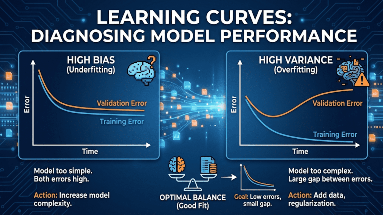
Pattern 1: High Bias (Underfitting)
What it looks like:
- Training score converges quickly and plateaus at a low/moderate level
- Validation score converges to the same low/moderate level
- The gap between the two curves is small (they meet early and stay close)
What it means: The model lacks the capacity to capture the complexity of the underlying relationship. Adding more training data will not help significantly — the curves have already converged, and the convergence point is the model’s ceiling. The model is not complex enough to benefit from additional examples.
Diagnosis confirmed by:
- Training accuracy of ~70% on 10,000 samples (not just 100)
- Validation accuracy matching training accuracy at that same low level
- No meaningful separation between the two curves
Fixes:
- Use a more complex model (more layers, more trees, higher-degree polynomial)
- Add more informative features
- Reduce regularization strength
Pattern 2: High Variance (Overfitting)
What it looks like:
- Training score starts high (often near 100%) and decreases slowly
- Validation score starts low and increases slowly
- A large, persistent gap remains between the two curves even at the largest training sizes
What it means: The model has memorized the training data rather than learning generalizable patterns. It performs excellently on examples it has seen but poorly on new examples. The gap represents the difference between memorization and genuine learning.
Diagnosis confirmed by:
- Training accuracy 95%, validation accuracy 75% at your full dataset size
- Gap does not close significantly as training size increases
- Training score decreasing gradually (model is fitting more noise as n grows)
Fixes:
- More data (if the curves have not yet converged, adding data will help close the gap)
- Stronger regularization
- Reduce model complexity
- Feature selection or dimensionality reduction
- Ensemble methods (bagging in particular reduces variance)
Pattern 3: Good Fit (Appropriate Model)
What it looks like:
- Training score starts high and decreases
- Validation score starts low and increases
- The two curves converge to a high, stable value
- The remaining gap at full training size is small
What it means: The model has appropriate complexity for the task. It generalizes well. Further improvement requires either more data (if the plateau hasn’t been reached), feature engineering, or a different model family.
Pattern 4: Need More Data (Curves Still Converging)
What it looks like:
- Both curves are still moving — training score still decreasing, validation still increasing
- The gap is moderate and has been steadily closing
- Neither curve has plateaued
What it means: The model has not yet seen enough data to reach its performance ceiling. Collecting more data will likely close the gap further and improve validation performance. This is the situation where the investment in more data collection has a clear expected payoff.
Python Implementation: Learning Curves from Scratch
Understanding how to build learning curves manually builds deeper intuition than calling library functions directly.
import numpy as np
import matplotlib.pyplot as plt
import matplotlib.gridspec as gridspec
from sklearn.datasets import make_classification, make_regression
from sklearn.linear_model import LogisticRegression, Ridge
from sklearn.ensemble import RandomForestClassifier, GradientBoostingClassifier
from sklearn.preprocessing import StandardScaler
from sklearn.pipeline import Pipeline
from sklearn.metrics import accuracy_score, f1_score
from sklearn.model_selection import StratifiedKFold, cross_val_score
import warnings
warnings.filterwarnings('ignore')


def compute_learning_curve(model, X, y, train_sizes, cv_folds=5,
                            scoring='accuracy', task='classification'):
    """
    Compute learning curve data from scratch.

    At each training size, performs cross-validation to estimate
    both training and validation performance.

    Args:
        model:       Scikit-learn compatible model
        X, y:        Full dataset
        train_sizes: Array of absolute or fractional training sizes
        cv_folds:    Number of CV folds for each size estimate
        scoring:     Metric name (sklearn string)
        task:        'classification' or 'regression'

    Returns:
        Dictionary with sizes, train_scores, val_scores arrays
    """
    from sklearn.model_selection import StratifiedKFold, KFold
    from sklearn.metrics import get_scorer

    n = len(y)

    # Convert fractional sizes to absolute if needed
    if all(0 < s <= 1 for s in train_sizes):
        train_sizes_abs = [max(cv_folds, int(s * n)) for s in train_sizes]
    else:
        train_sizes_abs = [int(s) for s in train_sizes]

    train_sizes_abs = sorted(set(train_sizes_abs))

    scorer = get_scorer(scoring)
    cv = (StratifiedKFold(n_splits=cv_folds, shuffle=True, random_state=42)
          if task == 'classification' else
          KFold(n_splits=cv_folds, shuffle=True, random_state=42))

    mean_train_scores = []
    std_train_scores  = []
    mean_val_scores   = []
    std_val_scores    = []
    actual_sizes      = []

    for size in train_sizes_abs:
        if size >= n:
            size = n

        fold_train_scores = []
        fold_val_scores   = []

        for train_idx, val_idx in cv.split(X, y):
            # Use only `size` samples from the training fold
            # (subsample from the training indices, not the full dataset)
            if size < len(train_idx):
                subsample_idx = np.random.choice(train_idx, size=size, replace=False)
            else:
                subsample_idx = train_idx

            X_train_sub = X[subsample_idx]
            y_train_sub = y[subsample_idx]
            X_val       = X[val_idx]
            y_val       = y[val_idx]

            import copy
            m = copy.deepcopy(model)
            m.fit(X_train_sub, y_train_sub)

            fold_train_scores.append(scorer(m, X_train_sub, y_train_sub))
            fold_val_scores.append(scorer(m, X_val, y_val))

        mean_train_scores.append(np.mean(fold_train_scores))
        std_train_scores.append(np.std(fold_train_scores))
        mean_val_scores.append(np.mean(fold_val_scores))
        std_val_scores.append(np.std(fold_val_scores))
        actual_sizes.append(size)

    return {
        'sizes':       np.array(actual_sizes),
        'train_mean':  np.array(mean_train_scores),
        'train_std':   np.array(std_train_scores),
        'val_mean':    np.array(mean_val_scores),
        'val_std':     np.array(std_val_scores),
    }


def plot_learning_curve(lc_data, title="Learning Curve", metric_name="Score",
                         figsize=(9, 6), ax=None, color_train='steelblue',
                         color_val='coral', show_std=True):
    """
    Plot a learning curve with confidence bands.

    Args:
        lc_data:     Output from compute_learning_curve()
        title:       Plot title
        metric_name: Name of the metric (y-axis label)
        figsize:     Figure size (if creating new figure)
        ax:          Existing axes to plot into (optional)
        show_std:    Whether to show ±1 std shading
    """
    if ax is None:
        fig, ax = plt.subplots(figsize=figsize)
        standalone = True
    else:
        standalone = False

    sizes = lc_data['sizes']

    # Training score
    ax.plot(sizes, lc_data['train_mean'], 'o-', color=color_train,
            linewidth=2.5, markersize=6, label='Training score')
    if show_std:
        ax.fill_between(sizes,
                        lc_data['train_mean'] - lc_data['train_std'],
                        lc_data['train_mean'] + lc_data['train_std'],
                        alpha=0.15, color=color_train)

    # Validation score
    ax.plot(sizes, lc_data['val_mean'], 's-', color=color_val,
            linewidth=2.5, markersize=6, label='Validation score')
    if show_std:
        ax.fill_between(sizes,
                        lc_data['val_mean'] - lc_data['val_std'],
                        lc_data['val_mean'] + lc_data['val_std'],
                        alpha=0.15, color=color_val)

    # Gap annotation at final point
    final_gap = lc_data['train_mean'][-1] - lc_data['val_mean'][-1]
    ax.annotate(f'Gap={final_gap:.3f}',
                xy=(sizes[-1], (lc_data['train_mean'][-1] + lc_data['val_mean'][-1]) / 2),
                xytext=(-60, 0), textcoords='offset points',
                fontsize=9, color='gray',
                arrowprops=dict(arrowstyle='->', color='gray', lw=1.2))

    ax.set_xlabel("Training Set Size", fontsize=12)
    ax.set_ylabel(metric_name, fontsize=12)
    ax.set_title(title, fontsize=13, fontweight='bold')
    ax.legend(fontsize=11, loc='center right')
    ax.grid(True, alpha=0.3)
    ax.set_ylim([0, 1.05])

    if standalone:
        plt.tight_layout()

    return ax


# Generate dataset for demonstrations
np.random.seed(42)
X_main, y_main = make_classification(
    n_samples=3000, n_features=20, n_informative=12,
    n_redundant=4, random_state=42
)

train_sizes = np.linspace(0.05, 0.95, 15)

print("Computing learning curves (this may take a moment)...")Demonstrating the Four Patterns
# ── Four canonical learning curve patterns ──────────────────

np.random.seed(42)

# Generate data
X_demo, y_demo = make_classification(
    n_samples=2000, n_features=20, n_informative=8,
    random_state=42
)

# Scale for linear models
scaler_demo = StandardScaler()
X_demo_s = scaler_demo.fit_transform(X_demo)

train_sizes_demo = np.array([50, 100, 200, 400, 700, 1000, 1400, 1800])

# Models representing four patterns
pattern_models = {
    "Pattern 1: Underfitting\n(Linear model on nonlinear data)": (
        LogisticRegression(C=0.001, max_iter=1000, random_state=42),
        X_demo_s
    ),
    "Pattern 2: Overfitting\n(Deep tree, minimal regularization)": (
        RandomForestClassifier(
            n_estimators=10, max_depth=None,
            min_samples_leaf=1, random_state=42
        ),
        X_demo
    ),
    "Pattern 3: Good Fit\n(Well-tuned Random Forest)": (
        RandomForestClassifier(
            n_estimators=100, max_depth=8,
            min_samples_leaf=5, random_state=42
        ),
        X_demo
    ),
    "Pattern 4: Need More Data\n(Gradient Boosting, small dataset)": (
        GradientBoostingClassifier(
            n_estimators=200, max_depth=5, random_state=42
        ),
        X_demo[:800]  # Artificially restrict to show still-converging curves
    ),
}

fig, axes = plt.subplots(2, 2, figsize=(16, 12))
axes = axes.flatten()

for ax, (pattern_name, (model, X_pat)) in zip(axes, pattern_models.items()):
    y_pat = y_demo[:len(X_pat)]
    sizes = np.linspace(50, int(len(X_pat) * 0.85), 8).astype(int)

    lc = compute_learning_curve(model, X_pat, y_pat, sizes,
                                 cv_folds=5, scoring='accuracy')

    plot_learning_curve(lc, title=pattern_name, metric_name="Accuracy", ax=ax)

    # Annotate the final gap with interpretation
    gap = lc['train_mean'][-1] - lc['val_mean'][-1]
    val_plateau = lc['val_mean'][-1]

    if gap < 0.03 and val_plateau < 0.80:
        diagnosis = "⚠ Underfitting: Both scores low, gap small"
        color_box = '#ffcccc'
    elif gap > 0.10:
        diagnosis = "⚠ Overfitting: Large persistent gap"
        color_box = '#ffe0cc'
    elif gap < 0.05 and val_plateau > 0.80:
        diagnosis = "✓ Good fit: High score, small gap"
        color_box = '#ccffcc'
    else:
        diagnosis = "→ Need more data: Gap still closing"
        color_box = '#cce0ff'

    ax.text(0.02, 0.05, diagnosis, transform=ax.transAxes,
            fontsize=9, verticalalignment='bottom',
            bbox=dict(boxstyle='round', facecolor=color_box, alpha=0.8))

plt.suptitle("The Four Fundamental Learning Curve Patterns",
             fontsize=15, fontweight='bold', y=1.01)
plt.tight_layout()
plt.savefig("learning_curve_patterns.png", dpi=150, bbox_inches='tight')
plt.show()
print("Saved: learning_curve_patterns.png")Using Scikit-learn’s Built-in Learning Curve
For production use, scikit-learn’s learning_curve function is optimized and convenient. It parallelizes computation and handles edge cases correctly.
from sklearn.model_selection import learning_curve
from sklearn.datasets import load_digits
from sklearn.svm import SVC
from sklearn.ensemble import GradientBoostingClassifier
from sklearn.linear_model import LogisticRegression
from sklearn.preprocessing import StandardScaler
from sklearn.pipeline import Pipeline
import numpy as np
import matplotlib.pyplot as plt


def plot_sklearn_learning_curve(estimator, X, y, title,
                                  train_sizes=np.linspace(0.1, 1.0, 10),
                                  cv=5, scoring='accuracy', n_jobs=-1,
                                  figsize=(9, 6)):
    """
    Plot a learning curve using sklearn's learning_curve function.
    Includes confidence bands (±1 std across folds).

    Args:
        estimator:   Fitted or unfitted sklearn estimator/pipeline
        X, y:        Full dataset
        title:       Plot title
        train_sizes: Array of training set size fractions
        cv:          Number of CV folds
        scoring:     Metric name
        n_jobs:      Parallel jobs (-1 = all cores)
    """
    train_sizes_abs, train_scores, val_scores = learning_curve(
        estimator, X, y,
        train_sizes=train_sizes,
        cv=cv,
        scoring=scoring,
        n_jobs=n_jobs,
        shuffle=True,
        random_state=42
    )

    train_mean = train_scores.mean(axis=1)
    train_std  = train_scores.std(axis=1)
    val_mean   = val_scores.mean(axis=1)
    val_std    = val_scores.std(axis=1)

    fig, ax = plt.subplots(figsize=figsize)

    ax.plot(train_sizes_abs, train_mean, 'o-', color='steelblue',
            linewidth=2.5, markersize=7, label='Training score')
    ax.fill_between(train_sizes_abs, train_mean - train_std,
                    train_mean + train_std, alpha=0.15, color='steelblue')

    ax.plot(train_sizes_abs, val_mean, 's-', color='coral',
            linewidth=2.5, markersize=7, label='Cross-validation score')
    ax.fill_between(train_sizes_abs, val_mean - val_std,
                    val_mean + val_std, alpha=0.15, color='coral')

    # Annotate convergence
    final_gap = train_mean[-1] - val_mean[-1]
    ax.set_xlabel("Training Set Size", fontsize=12)
    ax.set_ylabel(scoring.replace('_', ' ').title(), fontsize=12)
    ax.set_title(f"{title}\n(Final gap: {final_gap:.4f})",
                 fontsize=13, fontweight='bold')
    ax.legend(fontsize=11, loc='center right')
    ax.grid(True, alpha=0.3)

    plt.tight_layout()
    plt.savefig(f"lc_{title.replace(' ', '_').replace('/', '_')[:30]}.png", dpi=150)
    plt.show()

    print(f"\n  {title}")
    print(f"  Final training score:    {train_mean[-1]:.4f} ± {train_std[-1]:.4f}")
    print(f"  Final validation score:  {val_mean[-1]:.4f} ± {val_std[-1]:.4f}")
    print(f"  Gap (overfit indicator): {final_gap:.4f}")

    return train_sizes_abs, train_mean, val_mean


# Load digits dataset (1,797 samples, 64 features, 10 classes)
digits = load_digits()
X_dig, y_dig = digits.data, digits.target

print("=== Learning Curves: Digits Dataset ===\n")

# Compare three models
models_comparison = [
    ("Logistic Regression", Pipeline([
        ('scaler', StandardScaler()),
        ('clf', LogisticRegression(max_iter=1000, random_state=42))
    ])),
    ("SVM (RBF kernel)", Pipeline([
        ('scaler', StandardScaler()),
        ('clf', SVC(kernel='rbf', C=1.0, gamma='scale', random_state=42))
    ])),
    ("Gradient Boosting", GradientBoostingClassifier(
        n_estimators=100, max_depth=4, random_state=42
    )),
]

for title, model in models_comparison:
    plot_sklearn_learning_curve(
        model, X_dig, y_dig,
        title=title,
        train_sizes=np.linspace(0.05, 1.0, 12),
        cv=5, scoring='accuracy', n_jobs=-1
)Validation Curves: Diagnosing Hyperparameter Sensitivity
A closely related tool is the validation curve, which plots training and validation performance against a single hyperparameter value rather than against training set size. Where learning curves answer “how much data do I need?”, validation curves answer “what value of this hyperparameter is best?”
from sklearn.model_selection import validation_curve
from sklearn.ensemble import RandomForestClassifier
from sklearn.datasets import make_classification
import numpy as np
import matplotlib.pyplot as plt


def plot_validation_curve(estimator, X, y, param_name, param_range,
                           title, cv=5, scoring='accuracy', log_scale=False,
                           n_jobs=-1, figsize=(9, 6)):
    """
    Plot validation curve: training and CV score vs a hyperparameter.

    Reveals:
    - Underfitting region: low scores for both (parameter too constrained)
    - Overfitting region: high training, low validation (too unconstrained)
    - Sweet spot: both scores high and close together

    Args:
        param_name:  Name of the hyperparameter to vary
        param_range: Values to evaluate the parameter at
        log_scale:   Whether to use log scale on x-axis
    """
    train_scores, val_scores = validation_curve(
        estimator, X, y,
        param_name=param_name,
        param_range=param_range,
        cv=cv, scoring=scoring,
        n_jobs=n_jobs
    )

    train_mean = train_scores.mean(axis=1)
    train_std  = train_scores.std(axis=1)
    val_mean   = val_scores.mean(axis=1)
    val_std    = val_scores.std(axis=1)

    best_idx = np.argmax(val_mean)
    best_val = param_range[best_idx]

    fig, ax = plt.subplots(figsize=figsize)

    x_vals = np.log10(param_range) if log_scale else np.array(param_range, dtype=float)
    x_label = f"log10({param_name})" if log_scale else param_name

    ax.plot(x_vals, train_mean, 'o-', color='steelblue',
            linewidth=2.5, markersize=7, label='Training score')
    ax.fill_between(x_vals, train_mean - train_std, train_mean + train_std,
                    alpha=0.15, color='steelblue')

    ax.plot(x_vals, val_mean, 's-', color='coral',
            linewidth=2.5, markersize=7, label='Validation score')
    ax.fill_between(x_vals, val_mean - val_std, val_mean + val_std,
                    alpha=0.15, color='coral')

    # Mark optimal
    ax.axvline(x=x_vals[best_idx], color='green', linestyle='--', lw=2,
               label=f'Best {param_name}={best_val}')

    # Shade regions
    if len(x_vals) > 4:
        split_point = len(x_vals) // 3
        ax.axvspan(x_vals[0], x_vals[split_point], alpha=0.05, color='blue',
                   label='Underfitting region')
        ax.axvspan(x_vals[-split_point], x_vals[-1], alpha=0.05, color='red',
                   label='Overfitting region')

    ax.set_xlabel(x_label, fontsize=12)
    ax.set_ylabel(scoring.replace('_', ' ').title(), fontsize=12)
    ax.set_title(f"{title}\nBest {param_name}={best_val} (Val={val_mean[best_idx]:.4f})",
                 fontsize=12, fontweight='bold')
    ax.legend(fontsize=9, loc='lower right')
    ax.grid(True, alpha=0.3)

    plt.tight_layout()
    plt.savefig(f"vc_{param_name[:20]}.png", dpi=150)
    plt.show()

    print(f"  Best {param_name}: {best_val}  (Val score: {val_mean[best_idx]:.4f})")
    return best_val


np.random.seed(42)
X_vc, y_vc = make_classification(
    n_samples=1500, n_features=20, n_informative=12, random_state=42
)

print("=== Validation Curves ===\n")

# Validation curve for max_depth in Random Forest
from sklearn.ensemble import RandomForestClassifier
rf_vc = RandomForestClassifier(n_estimators=100, random_state=42, n_jobs=-1)

best_depth = plot_validation_curve(
    rf_vc, X_vc, y_vc,
    param_name='max_depth',
    param_range=[1, 2, 3, 5, 7, 10, 15, 20, None],
    title="Random Forest: max_depth Validation Curve",
    cv=5, scoring='accuracy'
)

# Validation curve for C in Logistic Regression
from sklearn.linear_model import LogisticRegression
from sklearn.preprocessing import StandardScaler
from sklearn.pipeline import Pipeline

lr_pipe = Pipeline([
    ('scaler', StandardScaler()),
    ('clf', LogisticRegression(max_iter=1000, random_state=42))
])

C_range = np.logspace(-4, 4, 20)
best_C = plot_validation_curve(
    lr_pipe, X_vc, y_vc,
    param_name='clf__C',
    param_range=C_range,
    title="Logistic Regression: Regularization (C) Validation Curve",
    cv=5, scoring='accuracy', log_scale=True
)Advanced Learning Curve Analysis
The Learning Rate of Improvement
Beyond the final gap, a key question is: how quickly is the validation score still improving? If the slope of the validation curve is still steep at your full data size, you are in the “need more data” regime. If it has flattened out, additional data will provide diminishing returns.
import numpy as np
import matplotlib.pyplot as plt
from sklearn.model_selection import learning_curve
from sklearn.ensemble import GradientBoostingClassifier
from sklearn.datasets import make_classification

def analyze_learning_rate(estimator, X, y, title="Model",
                            train_sizes=np.linspace(0.05, 1.0, 15),
                            cv=5, scoring='accuracy'):
    """
    Analyze the rate of improvement of the validation curve
    to determine if collecting more data would help.

    Fits a power law curve to the validation scores and
    extrapolates to estimate performance at larger data sizes.
    """
    from scipy.optimize import curve_fit

    sizes, train_scores, val_scores = learning_curve(
        estimator, X, y,
        train_sizes=train_sizes, cv=cv,
        scoring=scoring, n_jobs=-1,
        shuffle=True, random_state=42
    )

    val_mean   = val_scores.mean(axis=1)
    train_mean = train_scores.mean(axis=1)

    # Fit power law: score(n) = ceiling - (a / n^b)
    # This models the typical learning curve shape
    def power_law_model(n, ceiling, a, b):
        return ceiling - a / (n ** b)

    try:
        popt, _ = curve_fit(
            power_law_model, sizes, val_mean,
            p0=[val_mean[-1] + 0.05, 10, 0.5],
            bounds=([val_mean[-1], 0, 0], [1.0, 1000, 2.0]),
            maxfev=5000
        )
        ceiling, a, b = popt

        # Extrapolate to 2× and 5× current data
        n_current = sizes[-1]
        score_2x  = power_law_model(n_current * 2, *popt)
        score_5x  = power_law_model(n_current * 5, *popt)
        score_inf = ceiling

        # Improvement rate at current size
        improvement_slope = a * b / (n_current ** (b + 1))

        print(f"\n=== Learning Rate Analysis: {title} ===")
        print(f"  Current data size:     {n_current:,.0f} samples")
        print(f"  Current val score:     {val_mean[-1]:.4f}")
        print(f"\n  Extrapolated performance:")
        print(f"  At 2× data ({2*n_current:.0f}):  {min(score_2x, 1.0):.4f}")
        print(f"  At 5× data ({5*n_current:.0f}):  {min(score_5x, 1.0):.4f}")
        print(f"  Asymptotic ceiling:    {min(ceiling, 1.0):.4f}")
        print(f"\n  Improvement slope at current size: {improvement_slope:.6f} per sample")

        if improvement_slope > 0.0001:
            verdict = "📈 More data likely to help significantly"
        elif improvement_slope > 0.00001:
            verdict = "📊 More data may help modestly"
        else:
            verdict = "📉 Diminishing returns — model near its ceiling"

        print(f"  Verdict: {verdict}")

        # Plot with extrapolation
        fig, ax = plt.subplots(figsize=(10, 6))

        ax.plot(sizes, train_mean, 'o-', color='steelblue', lw=2.5,
                markersize=7, label='Training score')
        ax.plot(sizes, val_mean, 's-', color='coral', lw=2.5,
                markersize=7, label='Validation score')

        # Extrapolation curve
        n_extrap = np.linspace(sizes[0], sizes[-1] * 5, 200)
        score_extrap = np.clip(power_law_model(n_extrap, *popt), 0, 1)
        ax.plot(n_extrap, score_extrap, '--', color='green', lw=2,
                alpha=0.7, label=f'Extrapolation (ceiling≈{ceiling:.3f})')

        ax.axvline(x=n_current, color='gray', linestyle=':', lw=1.5,
                   label=f'Current size ({n_current:.0f})')
        ax.axhline(y=ceiling, color='green', linestyle=':', lw=1.5, alpha=0.5)

        # Mark extrapolated points
        for mult, score in [(2, score_2x), (5, score_5x)]:
            if n_current * mult <= n_extrap[-1]:
                ax.scatter(n_current * mult, min(score, 1.0),
                           color='green', s=150, zorder=5,
                           marker='^', label=f'{mult}× data: {min(score, 1.0):.4f}')

        ax.set_xlabel("Training Set Size", fontsize=12)
        ax.set_ylabel(scoring.replace('_', ' ').title(), fontsize=12)
        ax.set_title(f"{title}: Learning Rate & Extrapolation", fontsize=13, fontweight='bold')
        ax.legend(fontsize=9, loc='lower right')
        ax.grid(True, alpha=0.3)

        plt.tight_layout()
        plt.savefig("learning_rate_analysis.png", dpi=150)
        plt.show()
        print("  Saved: learning_rate_analysis.png")

    except Exception as e:
        print(f"  Power law fit failed: {e}. Reporting raw values only.")

    return sizes, train_mean, val_mean


np.random.seed(42)
X_lr, y_lr = make_classification(
    n_samples=5000, n_features=20, n_informative=14, random_state=42
)

gbm_lr = GradientBoostingClassifier(n_estimators=100, max_depth=5, random_state=42)
analyze_learning_rate(gbm_lr, X_lr, y_lr, title="Gradient Boosting")Learning Curves for Regression
Learning curves work identically for regression problems — the only difference is the metric (typically negative MSE or R²).
from sklearn.model_selection import learning_curve
from sklearn.ensemble import RandomForestRegressor, GradientBoostingRegressor
from sklearn.linear_model import LinearRegression, Ridge
from sklearn.datasets import fetch_california_housing
from sklearn.preprocessing import StandardScaler
from sklearn.pipeline import Pipeline
import numpy as np
import matplotlib.pyplot as plt

# California housing dataset
housing = fetch_california_housing()
X_hs, y_hs = housing.data, housing.target

print("=== Regression Learning Curves: California Housing ===\n")

reg_models = {
    "Linear Regression": Pipeline([
        ('scaler', StandardScaler()),
        ('reg', LinearRegression())
    ]),
    "Ridge Regression": Pipeline([
        ('scaler', StandardScaler()),
        ('reg', Ridge(alpha=1.0))
    ]),
    "Random Forest": RandomForestRegressor(100, random_state=42, n_jobs=-1),
    "Gradient Boosting": GradientBoostingRegressor(100, random_state=42),
}

fig, axes = plt.subplots(2, 2, figsize=(16, 12))
axes = axes.flatten()

for ax, (name, model) in zip(axes, reg_models.items()):
    sizes, train_sc, val_sc = learning_curve(
        model, X_hs, y_hs,
        train_sizes=np.linspace(0.05, 1.0, 12),
        cv=5, scoring='r2', n_jobs=-1,
        shuffle=True, random_state=42
    )

    train_mean = train_sc.mean(axis=1)
    val_mean   = val_sc.mean(axis=1)
    train_std  = train_sc.std(axis=1)
    val_std    = val_sc.std(axis=1)

    ax.plot(sizes, train_mean, 'o-', color='steelblue', lw=2.5,
            markersize=7, label='Training R²')
    ax.fill_between(sizes, train_mean - train_std, train_mean + train_std,
                    alpha=0.15, color='steelblue')

    ax.plot(sizes, val_mean, 's-', color='coral', lw=2.5,
            markersize=7, label='Validation R²')
    ax.fill_between(sizes, val_mean - val_std, val_mean + val_std,
                    alpha=0.15, color='coral')

    final_gap = train_mean[-1] - val_mean[-1]
    ax.set_xlabel("Training Set Size", fontsize=11)
    ax.set_ylabel("R² Score", fontsize=11)
    ax.set_title(f"{name}\n(Final Gap: {final_gap:.3f})",
                 fontsize=12, fontweight='bold')
    ax.legend(fontsize=9)
    ax.grid(True, alpha=0.3)
    ax.set_ylim([-0.2, 1.1])

    print(f"{name:<25}: Train R²={train_mean[-1]:.4f}, Val R²={val_mean[-1]:.4f}, "
          f"Gap={final_gap:.4f}")

plt.suptitle("Regression Learning Curves: California Housing Dataset",
             fontsize=14, fontweight='bold', y=1.01)
plt.tight_layout()
plt.savefig("regression_learning_curves.png", dpi=150, bbox_inches='tight')
plt.show()
print("\nSaved: regression_learning_curves.png")Using Learning Curves to Answer the “More Data?” Question
One of the most common and valuable uses of learning curves is answering a critical business question: “Should we invest in collecting more data?” This question has real cost implications — labeling medical images, conducting surveys, running experiments, or purchasing datasets all require time and money.
Learning curves give you a principled way to answer this before making the investment.
import numpy as np
import matplotlib.pyplot as plt
from sklearn.model_selection import learning_curve
from sklearn.ensemble import GradientBoostingClassifier, RandomForestClassifier
from sklearn.datasets import make_classification

def data_investment_analysis(estimator, X, y, current_n,
                              target_n_options, scoring='roc_auc',
                              cv=5, title="Model"):
    """
    Analyze whether collecting more data is likely to improve performance.

    Creates a learning curve up to current data size, extrapolates,
    and provides a recommendation with expected gains.

    Args:
        estimator:          Sklearn model
        X, y:               Current full dataset
        current_n:          Current training set size
        target_n_options:   List of potential future dataset sizes to evaluate
        scoring:            Evaluation metric
    """
    from scipy.optimize import curve_fit

    sizes, train_scores, val_scores = learning_curve(
        estimator, X, y,
        train_sizes=np.linspace(0.10, 1.0, 12),
        cv=cv, scoring=scoring, n_jobs=-1,
        shuffle=True, random_state=42
    )

    val_mean  = val_scores.mean(axis=1)
    train_mean = train_scores.mean(axis=1)

    current_val  = val_mean[-1]
    current_train = train_mean[-1]
    current_gap  = current_train - current_val

    # Determine diagnosis
    print(f"\n{'='*58}")
    print(f"  Data Investment Analysis: {title}")
    print(f"{'='*58}")
    print(f"\n  Current dataset: {current_n:,} samples")
    print(f"  Current training {scoring}: {current_train:.4f}")
    print(f"  Current validation {scoring}: {current_val:.4f}")
    print(f"  Gap: {current_gap:.4f}")

    # Diagnosis
    if current_gap > 0.10:
        print(f"\n  🔴 Diagnosis: HIGH VARIANCE (Overfitting)")
        print(f"  More data would help if the validation curve hasn't plateaued.")
        print(f"  Also consider: regularization, simpler model, feature reduction.")
    elif current_val < 0.70:
        print(f"\n  🔴 Diagnosis: HIGH BIAS (Underfitting)")
        print(f"  More data is unlikely to help significantly.")
        print(f"  Recommendation: Use a more complex model or add features.")
        return
    else:
        print(f"\n  🟢 Diagnosis: Generally good fit")

    # Slope at current point (improvement rate)
    if len(val_mean) >= 3:
        recent_slope = (val_mean[-1] - val_mean[-3]) / (sizes[-1] - sizes[-3])
        slope_per_1k = recent_slope * 1000
        print(f"\n  Learning rate: +{slope_per_1k:.4f} {scoring} per 1,000 additional samples")

        print(f"\n  Projected performance at target dataset sizes:")
        print(f"  {'Target Size':>15} | {'Expected Gain':>14} | {'Expected Score':>15} | Recommendation")
        print("  " + "-" * 65)

        for target_n in target_n_options:
            additional_n = target_n - current_n
            if additional_n <= 0:
                continue

            # Linear extrapolation (conservative estimate)
            expected_gain  = recent_slope * additional_n
            expected_score = min(current_val + expected_gain, 1.0)

            if expected_gain > 0.05:
                rec = "✓ Strongly recommended"
            elif expected_gain > 0.02:
                rec = "~ Consider if cost is low"
            else:
                rec = "✗ Diminishing returns"

            print(f"  {target_n:>15,} | {expected_gain:>+14.4f} | {expected_score:>15.4f} | {rec}")

    # Plot
    fig, ax = plt.subplots(figsize=(10, 6))
    ax.plot(sizes, train_mean, 'o-', color='steelblue', lw=2.5,
            markersize=7, label='Training score')
    ax.plot(sizes, val_mean, 's-', color='coral', lw=2.5,
            markersize=7, label='Validation score')

    # Extrapolation line
    if len(val_mean) >= 3:
        extrap_sizes = np.array([sizes[-1]] + target_n_options)
        extrap_scores = current_val + recent_slope * (extrap_sizes - sizes[-1])
        extrap_scores = np.clip(extrap_scores, 0, 1.0)
        ax.plot(extrap_sizes, extrap_scores, '--', color='green', lw=2,
                alpha=0.7, label='Extrapolated gain')

    ax.axvline(x=sizes[-1], color='gray', linestyle=':', lw=1.5, label='Current size')
    ax.set_xlabel("Training Set Size", fontsize=12)
    ax.set_ylabel(scoring.replace('_', ' ').upper(), fontsize=12)
    ax.set_title(f"Data Investment Analysis: {title}", fontsize=13, fontweight='bold')
    ax.legend(fontsize=10)
    ax.grid(True, alpha=0.3)
    plt.tight_layout()
    plt.savefig("data_investment_analysis.png", dpi=150)
    plt.show()
    print("\n  Saved: data_investment_analysis.png")


np.random.seed(42)
X_invest, y_invest = make_classification(
    n_samples=3000, n_features=20, n_informative=10,
    weights=[0.80, 0.20], random_state=42
)

gbm_invest = GradientBoostingClassifier(100, random_state=42)

data_investment_analysis(
    gbm_invest, X_invest, y_invest,
    current_n=3000,
    target_n_options=[5000, 10000, 20000, 50000],
    scoring='roc_auc',
    title="Gradient Boosting Classifier"
)Learning Curves Across Different Model Families
Different model families produce characteristically different learning curve shapes. Understanding these signatures helps you interpret curves quickly.
Decision Trees and Forests: Unconstrained decision trees overfit almost perfectly on small datasets (training score = 1.0) but generalize poorly. Ensemble methods (Random Forests, Gradient Boosting) show a more graceful curve: training score starts high but descends more gradually, and the validation score rises more steeply — thanks to variance reduction through averaging.
Linear Models: Logistic regression, linear regression, and ridge/lasso models show characteristic fast convergence. With just a few hundred samples, linear models often reach close to their asymptotic performance because they have few parameters to estimate. The gap between training and validation scores is typically small. The limitation shows up as a low-but-stable validation score — the model is not overfitting; it simply lacks capacity.
Neural Networks: Deep neural networks show the slowest convergence, requiring the most data before validation performance stabilizes. On very small datasets, deep networks typically overfit severely, showing near-perfect training scores with poor validation. As data scales into the tens or hundreds of thousands, the validation curve may still be rising — neural networks are among the few model types that genuinely benefit from millions of examples.
import numpy as np
import matplotlib.pyplot as plt
from sklearn.model_selection import learning_curve
from sklearn.linear_model import LogisticRegression
from sklearn.tree import DecisionTreeClassifier
from sklearn.ensemble import RandomForestClassifier, GradientBoostingClassifier
from sklearn.preprocessing import StandardScaler
from sklearn.pipeline import Pipeline
from sklearn.datasets import make_classification
import warnings
warnings.filterwarnings('ignore')

np.random.seed(42)
X_cmp, y_cmp = make_classification(
    n_samples=4000, n_features=20, n_informative=12,
    n_redundant=4, weights=[0.6, 0.4], random_state=42
)

model_signatures = {
    "Logistic Regression\n(Low variance, may underfit)": Pipeline([
        ('sc', StandardScaler()),
        ('clf', LogisticRegression(max_iter=1000, random_state=42))
    ]),
    "Decision Tree (max_depth=None)\n(High variance, severe overfit)":
        DecisionTreeClassifier(max_depth=None, random_state=42),
    "Random Forest\n(Balanced ensemble)":
        RandomForestClassifier(100, max_depth=8, random_state=42, n_jobs=-1),
    "Gradient Boosting\n(Strong learner, moderate variance)":
        GradientBoostingClassifier(100, max_depth=4, random_state=42),
}

fig, axes = plt.subplots(2, 2, figsize=(16, 11))
axes_flat = axes.flatten()
sizes_cmp = np.linspace(0.05, 1.0, 12)

for ax, (name, model) in zip(axes_flat, model_signatures.items()):
    sizes, tr_sc, va_sc = learning_curve(
        model, X_cmp, y_cmp,
        train_sizes=sizes_cmp, cv=5, scoring='roc_auc',
        n_jobs=-1, shuffle=True, random_state=42
    )

    tr_mean = tr_sc.mean(axis=1)
    va_mean = va_sc.mean(axis=1)
    tr_std  = tr_sc.std(axis=1)
    va_std  = va_sc.std(axis=1)

    ax.plot(sizes, tr_mean, 'o-', color='steelblue', lw=2.5, markersize=6, label='Train AUC')
    ax.fill_between(sizes, tr_mean-tr_std, tr_mean+tr_std, alpha=0.12, color='steelblue')
    ax.plot(sizes, va_mean, 's-', color='coral', lw=2.5, markersize=6, label='Val AUC')
    ax.fill_between(sizes, va_mean-va_std, va_mean+va_std, alpha=0.12, color='coral')

    gap = tr_mean[-1] - va_mean[-1]
    ax.set_xlabel("Training Set Size", fontsize=10)
    ax.set_ylabel("AUC-ROC", fontsize=10)
    ax.set_title(f"{name}\n(Final gap: {gap:.3f})", fontsize=10, fontweight='bold')
    ax.legend(fontsize=9)
    ax.grid(True, alpha=0.3)
    ax.set_ylim([0.45, 1.05])

plt.suptitle("Learning Curve Signatures by Model Family",
             fontsize=13, fontweight='bold', y=1.01)
plt.tight_layout()
plt.savefig("model_family_learning_curves.png", dpi=150, bbox_inches='tight')
plt.show()
print("Saved: model_family_learning_curves.png")The Bayes Error Rate and the Performance Ceiling
Every learning curve has a ceiling it cannot exceed — the Bayes error rate. This is the irreducible error that remains even with infinite data and an optimal model. It arises from noise in labels, missing features that are genuinely required to make perfect predictions, and inherent randomness in the process being modeled.
Understanding the Bayes error rate prevents a common mistake: spending enormous effort trying to close a gap that is actually irreducible. If the best human experts achieve 85% accuracy on your task, a model achieving 83% validation accuracy with a 2% gap to training is performing near-optimally — not overfitting.
How do you estimate the Bayes error? Three main approaches:
Human expert performance: For tasks with human-interpretable inputs, domain experts set the practical ceiling. If radiologists reading chest X-rays achieve 92% sensitivity, a model at 91% is near the ceiling — a model at 85% still has room to grow.
Noise analysis: If your labels have annotation noise (disagreement between raters), that noise rate is a lower bound on the error rate any model can achieve. A dataset where raters agree only 90% of the time cannot be classified with more than ~90% accuracy on average.
Irreducible class overlap: For tabular data, if two classes have identical feature distributions for some fraction of samples, perfect classification is mathematically impossible. Label entropy analysis reveals this.
The key practical implication: if your validation curve has plateaued and the gap to training is small, check whether your validation performance is close to human-level or near any known noise ceiling. If it is, you have likely found the Bayes error floor — further investment in data or model complexity will not help.
A Diagnostic Framework: Reading Any Learning Curve
When you generate a learning curve, work through this systematic diagnostic:
Step 1: Look at the training score at your full dataset size
        │
        ├─ Very high (>95%)?   → Likely overfitting, check the gap
        ├─ Moderate (70-85%)?  → Could be appropriate, check the gap
        └─ Low (<70%)?         → Likely underfitting, model too simple

Step 2: Look at the validation score at your full dataset size
        │
        ├─ Close to training?  → Good sign (convergence)
        └─ Far below training? → Overfitting — measure the gap

Step 3: Measure the gap (training − validation) at full size
        │
        ├─ Gap < 3%            → Healthy model
        ├─ Gap 3-10%           → Moderate overfitting, try regularization
        └─ Gap > 10%           → Significant overfitting

Step 4: Look at the slope of the validation curve at the right edge
        │
        ├─ Still rising steeply? → More data will help
        ├─ Flattening out?       → Near plateau, diminishing returns
        └─ Completely flat?      → More data won't help

Step 5: Determine the fix
        │
        ├─ Underfitting + small gap:
        │    → More complex model, more features, less regularization
        │
        ├─ Overfitting + large gap + validation still rising:
        │    → Collect more data (primary fix)
        │    → Also try: regularization, dropout, feature selection
        │
        ├─ Overfitting + large gap + validation plateaued:
        │    → More data won't help: use regularization, ensemble, simpler model
        │
        └─ Good fit + high scores:
→ You're done! Or fine-tune hyperparameters for marginal gain.def diagnose_learning_curve(train_scores, val_scores, sizes, metric_name="score"):
"""
Automated learning curve diagnosis.
Args:
train_scores: Array of training scores across sizes
val_scores: Array of validation scores across sizes
sizes: Array of corresponding training sizes
Returns:
Dictionary with diagnosis and recommendations
"""
final_train = train_scores[-1]
final_val = val_scores[-1]
gap = final_train - final_val
# Compute slope at the right end (last 3 points)
if len(val_scores) >= 3:
slope = (val_scores[-1] - val_scores[-3]) / (sizes[-1] - sizes[-3])
slope_per_1k = slope * 1000
else:
slope = 0
slope_per_1k = 0
# Diagnose
issues = []
recommendations = []
if final_val < 0.65:
issues.append("HIGH BIAS: Validation score is low")
recommendations.append("Use a more complex model")
recommendations.append("Add more informative features")
recommendations.append("Reduce regularization strength")
if gap > 0.10:
issues.append(f"HIGH VARIANCE: Large train-val gap ({gap:.3f})")
if slope_per_1k > 0.001:
recommendations.append("Collect more training data (validation still improving)")
else:
recommendations.append("More data unlikely to help (validation plateaued)")
recommendations.append("Increase regularization strength")
recommendations.append("Reduce model complexity")
recommendations.append("Apply feature selection")
elif gap < 0.03 and final_val > 0.80:
issues.append("HEALTHY: Good fit with high score")
recommendations.append("Consider fine-tuning hyperparameters")
recommendations.append("Feature engineering for marginal gains")
if slope_per_1k > 0.005:
issues.append(f"STILL LEARNING: Validation improving rapidly ({slope_per_1k:.4f}/1k samples)")
recommendations.append("Collecting more data expected to yield measurable improvement")
print(f"\n=== Automated Learning Curve Diagnosis ===\n")
print(f" Training {metric_name} (final): {final_train:.4f}")
print(f" Validation {metric_name} (final): {final_val:.4f}")
print(f" Gap: {gap:.4f}")
print(f" Improvement slope: {slope_per_1k:+.5f} per 1,000 samples")
print(f"\n Issues detected:")
for issue in issues:
print(f" • {issue}")
print(f"\n Recommendations:")
for rec in recommendations:
print(f" → {rec}")
return {
"final_train": final_train,
"final_val": final_val,
"gap": gap,
"slope_per_1k": slope_per_1k,
"issues": issues,
"recommendations": recommendations
}Summary
Learning curves are one of the most informative diagnostic tools in the machine learning practitioner’s toolkit. By systematically varying training set size and measuring both training and validation performance, they reveal the true nature of a model’s struggle in a way that no single metric ever can.
The four fundamental patterns — underfitting (both curves plateau low), overfitting (large persistent gap), good fit (high convergence), and needing more data (curves still converging) — cover nearly every situation you will encounter in practice. Each pattern points directly to a specific class of remedies, making learning curves not just diagnostic but prescriptive.
Validation curves extend this concept to hyperparameter space, answering the complementary question: at what value does this parameter transition from underfitting to good fit to overfitting?
The “more data?” question deserves special attention. Before investing in expensive data collection, labeling, or acquisition, a learning curve on your current data gives you a principled extrapolation of likely gains. A validation curve that is still rising steeply at your current data boundary is a strong signal that data investment will pay off. A plateau is a strong signal it will not.
Together, learning curves and validation curves form a complete diagnostic system for understanding model behavior — turning the opaque process of “why doesn’t my model work well?” into a structured, evidence-based investigation.