Cross-validation is a technique for estimating how well a machine learning model will generalize to new, unseen data by systematically partitioning the available data into training and validation sets multiple times. The most common method, K-Fold cross-validation, splits data into K equal parts, trains on K-1 parts, and evaluates on the remaining part — repeating this K times so every sample is used for both training and validation. Cross-validation produces more reliable performance estimates than a single train-test split, especially on small datasets.
Introduction
You train a logistic regression model to detect email spam and evaluate it on a held-out test set. It achieves 94% accuracy. You train a random forest on the same data — 91% accuracy on the same test set. You choose logistic regression and deploy it.
But here is a question that should nag at you: how much of that 3-percentage-point difference is genuine, and how much is luck? With a single test set, a model can look good or bad simply because the specific 20% of samples that happened to land in the test set were unusually easy or hard. One particularly tricky batch of spam emails — or their absence — can swing your accuracy estimate by several percentage points.
This is the problem that cross-validation solves. Instead of evaluating your model on one specific test partition, cross-validation evaluates it on many different partitions systematically. The result is a much more reliable, less noisy estimate of your model’s true generalization performance — along with a quantification of how much that estimate varies.
This article covers the full spectrum of cross-validation strategies — from the foundational K-Fold method through specialized techniques for imbalanced data, time series, grouped data, nested hyperparameter tuning, and very small datasets. For each strategy, we explain when to use it, how it works, and provide complete Python implementations.
Why a Single Train-Test Split Is Not Enough
The Variance Problem
Consider splitting your dataset randomly into 80% training and 20% test. With 1,000 samples, your test set has 200 samples. On 200 samples, a 3% difference in accuracy corresponds to just 6 predictions. Six predictions going different ways due to which specific samples happened to land in the test set can make a better model look worse than an inferior one.
import numpy as np
import matplotlib.pyplot as plt
from sklearn.datasets import make_classification
from sklearn.linear_model import LogisticRegression
from sklearn.model_selection import train_test_split
from sklearn.preprocessing import StandardScaler

# Demonstrate variance in single-split evaluation
np.random.seed(0)
X, y = make_classification(
    n_samples=1000, n_features=15, n_informative=8,
    random_state=42
)

scaler = StandardScaler()
X_scaled = scaler.fit_transform(X)

# Repeat the same experiment with 50 different random seeds
accuracy_scores = []
for seed in range(50):
    X_tr, X_te, y_tr, y_te = train_test_split(
        X_scaled, y, test_size=0.2, random_state=seed
    )
    model = LogisticRegression(random_state=42, max_iter=1000)
    model.fit(X_tr, y_tr)
    accuracy_scores.append(model.score(X_te, y_te))

accuracy_scores = np.array(accuracy_scores)

print("=== Single Train-Test Split: Variance Demonstration ===\n")
print(f"  Accuracy across 50 different random splits:")
print(f"  Mean:   {accuracy_scores.mean():.4f}")
print(f"  Std:    {accuracy_scores.std():.4f}")
print(f"  Min:    {accuracy_scores.min():.4f}")
print(f"  Max:    {accuracy_scores.max():.4f}")
print(f"  Range:  {accuracy_scores.max() - accuracy_scores.min():.4f}")
print(f"\n  The same model varies by {(accuracy_scores.max() - accuracy_scores.min())*100:.1f}pp")
print(f"  across different random splits — just from sampling variation!")

# Visualize the distribution of single-split scores
plt.figure(figsize=(10, 4))
plt.hist(accuracy_scores, bins=15, edgecolor='white', color='steelblue', alpha=0.8)
plt.axvline(accuracy_scores.mean(), color='red', linestyle='--', lw=2,
            label=f'Mean={accuracy_scores.mean():.3f}')
plt.axvline(accuracy_scores.mean() - accuracy_scores.std(), color='orange',
            linestyle=':', lw=1.5, label=f'±1 std')
plt.axvline(accuracy_scores.mean() + accuracy_scores.std(), color='orange',
            linestyle=':', lw=1.5)
plt.xlabel("Test Accuracy (single split)", fontsize=12)
plt.ylabel("Frequency", fontsize=12)
plt.title("Distribution of Accuracy Scores Across 50 Random Train-Test Splits\n"
          "(Same model, same data — only the split changes)", fontsize=12, fontweight='bold')
plt.legend(fontsize=10)
plt.grid(True, alpha=0.3)
plt.tight_layout()
plt.savefig("single_split_variance.png", dpi=150)
plt.show()
print("Saved: single_split_variance.png")This simulation demonstrates that even with 1,000 samples, the same model can produce accuracy estimates spanning several percentage points just from split variability. Cross-validation addresses this by averaging over multiple such evaluations.
The Data Efficiency Problem
A single 80/20 split uses only 20% of your data for evaluation. Every sample that lands in the test set contributes nothing to training. Cross-validation allows every sample to participate in both training and evaluation at different points, making much more efficient use of limited data.
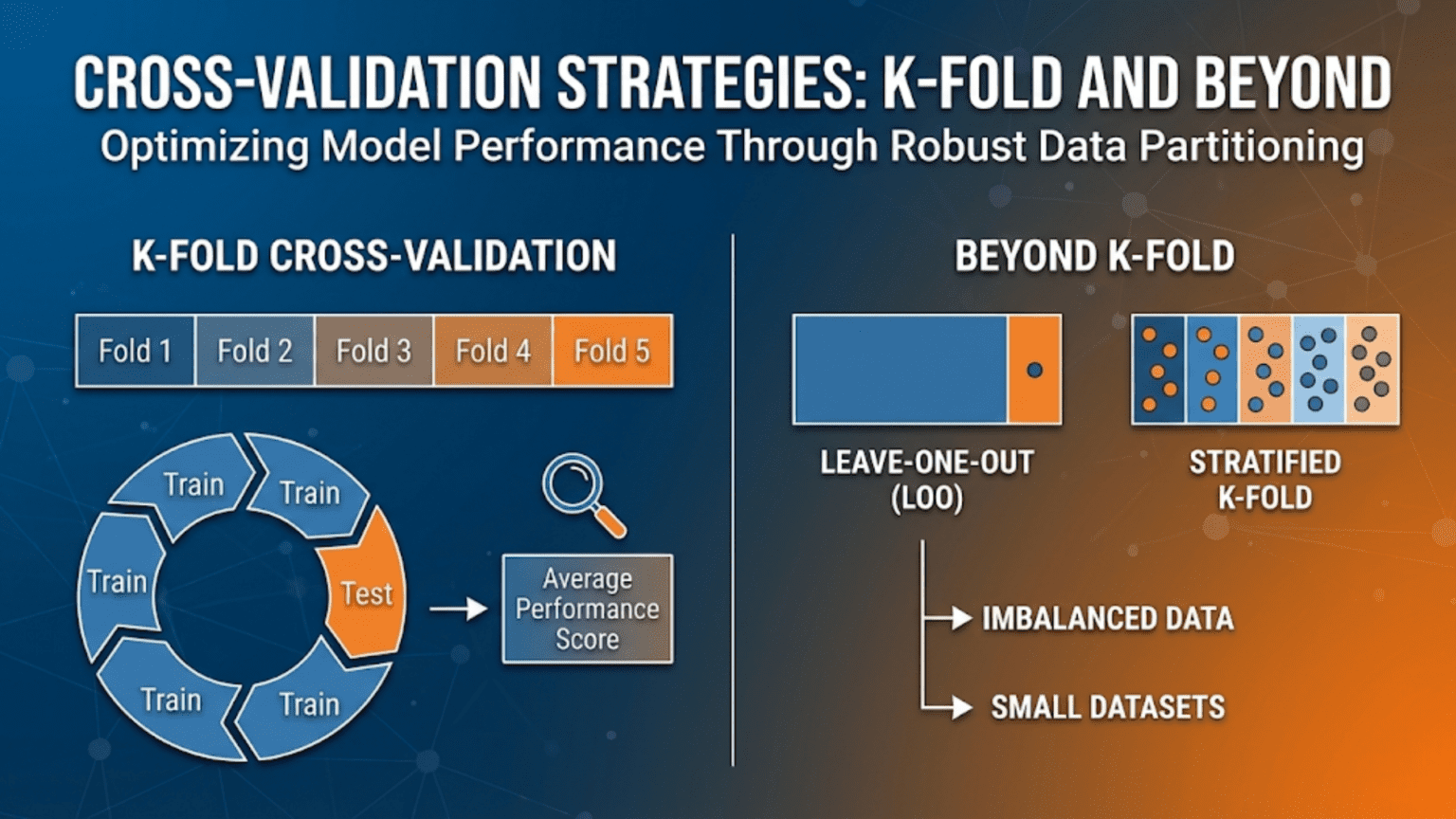
K-Fold Cross-Validation: The Foundation
How It Works
K-Fold cross-validation divides the dataset into K equal-sized subsets called folds. The procedure then:
- Holds out fold 1 as the validation set; trains on folds 2 through K
- Holds out fold 2 as the validation set; trains on folds 1, 3 through K
- Continues until each fold has been the validation set exactly once
- Reports the average performance across all K evaluations
With K=5, you train 5 models, each on 80% of the data and evaluated on a fresh 20%. With K=10, you train 10 models, each on 90% of the data and evaluated on a fresh 10%.
K = 5:
Fold 1: [TEST ] [TRAIN] [TRAIN] [TRAIN] [TRAIN]
Fold 2: [TRAIN] [TEST ] [TRAIN] [TRAIN] [TRAIN]
Fold 3: [TRAIN] [TRAIN] [TEST ] [TRAIN] [TRAIN]
Fold 4: [TRAIN] [TRAIN] [TRAIN] [TEST ] [TRAIN]
Fold 5: [TRAIN] [TRAIN] [TRAIN] [TRAIN] [TEST ]Choosing K
The choice of K involves a bias-variance tradeoff in the evaluation itself:
- Small K (e.g., K=3): Each training set is smaller (67% of data), so models see less training data. Performance is slightly underestimated (pessimistic bias). But computation is faster and variance across folds is lower.
- Large K (e.g., K=10): Each training set is larger (90% of data), giving a less biased estimate. But more variance across folds (each test fold is small) and higher computational cost.
- K=5 or K=10: The two most common choices. K=5 is popular for computational efficiency; K=10 is the traditional choice in academia for a good bias-variance balance.
from sklearn.model_selection import KFold, cross_val_score
from sklearn.datasets import make_classification
from sklearn.linear_model import LogisticRegression
from sklearn.preprocessing import StandardScaler
from sklearn.pipeline import Pipeline
import numpy as np

# Load our classification dataset
np.random.seed(42)
X, y = make_classification(
    n_samples=1000, n_features=15, n_informative=8, random_state=42
)

# Pipeline combines scaling + model cleanly for cross-validation
pipeline = Pipeline([
    ('scaler', StandardScaler()),
    ('classifier', LogisticRegression(random_state=42, max_iter=1000))
])

print("=== Effect of K on Cross-Validation Estimates ===\n")
print(f"{'K':>4} | {'Mean Accuracy':>14} | {'Std Dev':>9} | {'95% CI':>22} | {'Num Folds'}")
print("-" * 70)

for k in [2, 3, 5, 10, 20, 50]:
    kf = KFold(n_splits=k, shuffle=True, random_state=42)
    scores = cross_val_score(pipeline, X, y, cv=kf, scoring='accuracy')
    mean = scores.mean()
    std  = scores.std()
    ci_low  = mean - 1.96 * std / np.sqrt(k)
    ci_high = mean + 1.96 * std / np.sqrt(k)

    print(f"{k:>4} | {mean:>14.4f} | {std:>9.4f} | [{ci_low:.4f}, {ci_high:.4f}] | {k}")

print("\nNote: K=5 and K=10 provide reliable, efficient estimates.")
print("Very large K is computationally expensive with minimal benefit.")Complete K-Fold Implementation
from sklearn.model_selection import KFold, StratifiedKFold, cross_validate
from sklearn.ensemble import RandomForestClassifier, GradientBoostingClassifier
from sklearn.linear_model import LogisticRegression
from sklearn.metrics import make_scorer, accuracy_score, f1_score, roc_auc_score
from sklearn.preprocessing import StandardScaler
from sklearn.pipeline import Pipeline
import numpy as np

def comprehensive_cross_validation(models_dict, X, y, cv_strategy, cv_name,
                                    scoring_metrics=None):
    """
    Run cross-validation for multiple models and report comprehensive results.

    Args:
        models_dict:     Dict of {name: pipeline_or_model}
        X, y:            Features and labels
        cv_strategy:     Scikit-learn cross-validator object
        cv_name:         Display name for the CV strategy
        scoring_metrics: Dict of {metric_name: scorer}

    Returns:
        Results dictionary
    """
    if scoring_metrics is None:
        scoring_metrics = {
            'accuracy':  make_scorer(accuracy_score),
            'f1':        make_scorer(f1_score, zero_division=0),
            'roc_auc':   make_scorer(roc_auc_score, needs_proba=True),
        }

    print(f"\n{'='*65}")
    print(f"  Cross-Validation Strategy: {cv_name}")
    print(f"{'='*65}")

    all_results = {}

    for model_name, model in models_dict.items():
        cv_results = cross_validate(
            model, X, y,
            cv=cv_strategy,
            scoring=scoring_metrics,
            return_train_score=True,
            n_jobs=-1
        )

        all_results[model_name] = cv_results

        print(f"\n  {model_name}:")
        for metric in scoring_metrics:
            test_scores  = cv_results[f'test_{metric}']
            train_scores = cv_results[f'train_{metric}']

            mean_test = test_scores.mean()
            std_test  = test_scores.std()
            mean_train = train_scores.mean()

            overfit_gap = mean_train - mean_test

            print(f"    {metric:<10}: Test={mean_test:.4f}±{std_test:.4f}  "
                  f"Train={mean_train:.4f}  Gap={overfit_gap:+.4f}")

    return all_results


# Setup models
np.random.seed(42)
X, y = make_classification(
    n_samples=1500, n_features=20, n_informative=12,
    weights=[0.65, 0.35], random_state=42
)

models = {
    "Logistic Regression": Pipeline([
        ('scaler', StandardScaler()),
        ('clf', LogisticRegression(random_state=42, max_iter=1000))
    ]),
    "Random Forest": RandomForestClassifier(100, random_state=42, n_jobs=-1),
    "Gradient Boosting": GradientBoostingClassifier(100, random_state=42),
}

# Standard K-Fold
kf = KFold(n_splits=5, shuffle=True, random_state=42)
results_kf = comprehensive_cross_validation(models, X, y, kf, "5-Fold CV")Stratified K-Fold: Preserving Class Distribution
The Problem with Plain K-Fold on Classification
Ordinary K-Fold performs random splits without regard to class labels. On imbalanced datasets, some folds can end up with very few (or even zero) minority class samples — making the evaluation on those folds meaningless or numerically unstable.
Consider a dataset with 95% class 0 and 5% class 1, split into 10 folds. By chance, some folds might have only 1–2 positive samples, or none at all. Metrics like AUC and F1 become unreliable or undefined.
Stratified K-Fold: The Solution
Stratified K-Fold ensures each fold contains approximately the same proportion of each class as the full dataset. It achieves this by sampling from each class separately when constructing folds.
from sklearn.model_selection import StratifiedKFold, KFold
import numpy as np

def compare_fold_class_distributions(X, y, k=5, random_state=42):
    """
    Compare class distributions across folds for KFold vs StratifiedKFold.
    Shows why stratification matters for imbalanced datasets.
    """
    print("=== Class Distribution Across Folds ===\n")
    print(f"Overall class distribution: "
          f"Class 0={np.mean(y==0)*100:.1f}%, Class 1={np.mean(y==1)*100:.1f}%")

    for cv_class, cv_name in [
        (KFold(n_splits=k, shuffle=True, random_state=random_state), "Plain KFold"),
        (StratifiedKFold(n_splits=k, shuffle=True, random_state=random_state), "Stratified KFold"),
    ]:
        print(f"\n  {cv_name}:")
        print(f"  {'Fold':>6} | {'N Test':>8} | {'Class 0%':>9} | {'Class 1%':>9} | Status")
        print("  " + "-" * 50)

        class1_ratios = []
        for fold_i, (train_idx, test_idx) in enumerate(cv_class.split(X, y), 1):
            y_test_fold = y[test_idx]
            c0_pct = np.mean(y_test_fold == 0) * 100
            c1_pct = np.mean(y_test_fold == 1) * 100
            class1_ratios.append(c1_pct)

            # Flag if class 1 is underrepresented by more than 2%
            overall_c1 = np.mean(y == 1) * 100
            status = "⚠ Imbalanced" if abs(c1_pct - overall_c1) > 2 else "✓ Balanced"

            print(f"  {fold_i:>6} | {len(test_idx):>8} | {c0_pct:>8.1f}% | {c1_pct:>8.1f}% | {status}")

        print(f"  Std of Class 1% across folds: {np.std(class1_ratios):.2f}pp "
              f"({'low = good' if np.std(class1_ratios) < 1 else 'high = problem'})")


# Imbalanced dataset: 90% class 0, 10% class 1
X_imb, y_imb = make_classification(
    n_samples=500, n_features=10, n_informative=6,
    weights=[0.90, 0.10], random_state=42
)

compare_fold_class_distributions(X_imb, y_imb, k=5)Rule of thumb: Always use StratifiedKFold for classification problems. Scikit-learn’s cross_val_score and cross_validate functions automatically apply stratification when you pass a classifier — but it is good practice to set it explicitly, especially for imbalanced data.
Leave-One-Out Cross-Validation (LOO-CV)
What It Is
Leave-One-Out Cross-Validation is the extreme case of K-Fold where K = N (the number of samples). In each iteration, exactly one sample is held out as the test set, and the model is trained on all remaining N-1 samples.
When to Use LOO-CV
LOO-CV is most appropriate for very small datasets (typically fewer than 50–100 samples) where you cannot afford to leave out more than one sample at a time for evaluation.
from sklearn.model_selection import LeaveOneOut, cross_val_score
import numpy as np

# LOO-CV is most relevant for very small datasets
# Simulate a small medical study: 30 patients
np.random.seed(42)
X_small, y_small = make_classification(
    n_samples=30, n_features=8, n_informative=5, random_state=42
)

loo = LeaveOneOut()

print("=== Leave-One-Out Cross-Validation ===\n")
print(f"  Dataset: {len(y_small)} samples, {X_small.shape[1]} features")
print(f"  Number of CV iterations: {loo.get_n_splits(X_small)}")

pipeline_small = Pipeline([
    ('scaler', StandardScaler()),
    ('clf', LogisticRegression(random_state=42, max_iter=1000))
])

loo_scores = cross_val_score(pipeline_small, X_small, y_small,
                              cv=loo, scoring='accuracy')

print(f"\n  LOO-CV Accuracy: {loo_scores.mean():.4f} ± {loo_scores.std():.4f}")
print(f"  Individual fold scores (each is 0 or 1 since test size=1):")
print(f"  {loo_scores[:20].tolist()}...")

# Compare with K-Fold on same small data
for k in [3, 5, 10]:
    kf = StratifiedKFold(n_splits=min(k, y_small.sum()), shuffle=True, random_state=42)
    kf_scores = cross_val_score(pipeline_small, X_small, y_small,
                                 cv=kf, scoring='accuracy')
    print(f"\n  {k}-Fold CV Accuracy:  {kf_scores.mean():.4f} ± {kf_scores.std():.4f}")

print("\n  Recommendation: For n<50, LOO-CV or K=5 with small K correction.")
print(" LOO-CV is unbiased but has high variance — use it when data is very limited.")Tradeoffs of LOO-CV
| Aspect | LOO-CV | K-Fold |
|---|---|---|
| Bias | Very low (trains on N-1 samples each time) | Slightly higher |
| Variance | High (each test set is 1 sample) | Lower (each test set is N/K samples) |
| Computational cost | Very high (N model fits) | Moderate (K model fits) |
| Best for | Very small datasets (<50 samples) | Most practical scenarios |
Leave-P-Out Cross-Validation
A generalization of LOO-CV where P samples are held out in each iteration. With N=100 and P=2, there are C(100,2) = 4,950 iterations — computationally prohibitive. In practice, LOO (P=1) or K-Fold is used instead. Leave-P-Out is primarily a theoretical construct.
Repeated K-Fold: Reducing Variance Further
Standard K-Fold produces different results depending on how the data was shuffled before splitting. Repeated K-Fold runs the entire K-Fold procedure multiple times with different random shuffles, averaging results across all repetitions.
from sklearn.model_selection import RepeatedStratifiedKFold, RepeatedKFold
import numpy as np

np.random.seed(42)
X, y = make_classification(
    n_samples=500, n_features=15, n_informative=10, random_state=42
)

pipeline_rep = Pipeline([
    ('scaler', StandardScaler()),
    ('clf', LogisticRegression(random_state=42, max_iter=1000))
])

print("=== Repeated K-Fold: Reducing Variance in CV Estimates ===\n")
print(f"{'Strategy':<35} | {'Mean Acc':>9} | {'Std Dev':>9} | {'Num Evals'}")
print("-" * 65)

cv_strategies = [
    (StratifiedKFold(n_splits=5, shuffle=True, random_state=42),
     "5-Fold (single run)",         5),
    (RepeatedStratifiedKFold(n_splits=5, n_repeats=3, random_state=42),
     "5-Fold × 3 repeats",          15),
    (RepeatedStratifiedKFold(n_splits=5, n_repeats=10, random_state=42),
     "5-Fold × 10 repeats",         50),
    (RepeatedStratifiedKFold(n_splits=10, n_repeats=5, random_state=42),
     "10-Fold × 5 repeats",         50),
]

for cv, name, n_evals in cv_strategies:
    scores = cross_val_score(pipeline_rep, X, y, cv=cv, scoring='accuracy')
    print(f"{name:<35} | {scores.mean():>9.4f} | {scores.std():>9.4f} | {n_evals}")

print("\nMore repeats → lower std → more reliable estimate.")
print("Tradeoff: computation grows linearly with repeats.")Time Series Cross-Validation: Respecting Temporal Order
Standard K-Fold randomly shuffles data before splitting. For time series data, this is a serious mistake: it creates data leakage by allowing future information to appear in the training set of earlier periods. A model that “learns” from the future will appear to perform very well in cross-validation while failing completely in deployment.
Time Series Split
TimeSeriesSplit from scikit-learn creates an expanding window: each successive fold includes more historical data in training and evaluates on the next time window.
from sklearn.model_selection import TimeSeriesSplit
import numpy as np
import matplotlib.pyplot as plt

def visualize_time_series_splits(n_samples=200, n_splits=5):
    """
    Visualize how TimeSeriesSplit creates train/test windows.
    Shows why temporal order must be preserved.
    """
    tscv = TimeSeriesSplit(n_splits=n_splits)
    indices = np.arange(n_samples)

    fig, ax = plt.subplots(figsize=(12, 5))

    colors_train = plt.cm.Blues(np.linspace(0.3, 0.8, n_splits))
    colors_test  = plt.cm.Reds(np.linspace(0.5, 0.9, n_splits))

    for fold_i, (train_idx, test_idx) in enumerate(tscv.split(indices)):
        y_pos = n_splits - fold_i

        ax.barh(y_pos, len(train_idx), left=train_idx[0],
                height=0.4, color=colors_train[fold_i],
                label='Training' if fold_i == 0 else "")
        ax.barh(y_pos, len(test_idx), left=test_idx[0],
                height=0.4, color=colors_test[fold_i],
                label='Validation' if fold_i == 0 else "")
        ax.text(train_idx[0] + len(train_idx)/2, y_pos, f'Train ({len(train_idx)})',
                ha='center', va='center', fontsize=8, color='white', fontweight='bold')
        ax.text(test_idx[0] + len(test_idx)/2, y_pos, f'Test ({len(test_idx)})',
                ha='center', va='center', fontsize=8, color='white', fontweight='bold')
        ax.text(-2, y_pos, f'Fold {fold_i+1}', ha='right', va='center', fontsize=10)

    ax.set_xlabel("Time Index →", fontsize=12)
    ax.set_ylabel("Fold", fontsize=12)
    ax.set_title("Time Series Split: Training Always Precedes Validation\n"
                 "(Never training on future data to predict the past)",
                 fontsize=12, fontweight='bold')
    ax.legend(fontsize=10, loc='upper left')
    ax.set_xlim(-5, n_samples + 5)
    ax.set_yticks([])
    ax.grid(True, alpha=0.2, axis='x')
    plt.tight_layout()
    plt.savefig("time_series_cv_splits.png", dpi=150)
    plt.show()
    print("Saved: time_series_cv_splits.png")

visualize_time_series_splits()

# Practical time series cross-validation
from sklearn.model_selection import TimeSeriesSplit, cross_val_score
from sklearn.ensemble import GradientBoostingRegressor
from sklearn.metrics import make_scorer, mean_absolute_error

def create_time_series_features(n=1000):
    """Generate a synthetic time series with trend and seasonality."""
    np.random.seed(42)
    t = np.arange(n)

    # Signal: trend + seasonality + noise
    y = (0.05 * t                         # Linear trend
         + 10 * np.sin(2 * np.pi * t / 52) # Annual cycle (52 weeks)
         + 5  * np.sin(2 * np.pi * t / 12) # Monthly cycle
         + np.random.normal(0, 3, n))       # Noise

    # Features: lagged values (autoregressive features)
    lags = [1, 2, 4, 8, 12, 24, 52]
    X = np.column_stack([
        np.roll(y, lag) for lag in lags
    ])

    # Remove samples where lags reference nonexistent past data
    start = max(lags)
    return X[start:], y[start:]

X_ts, y_ts = create_time_series_features()

print(f"\n=== Time Series Cross-Validation ===\n")
print(f"Time series dataset: {len(y_ts)} timesteps, {X_ts.shape[1]} lag features\n")

tscv = TimeSeriesSplit(n_splits=5)
mae_scorer = make_scorer(mean_absolute_error, greater_is_better=False)

gbm_ts = GradientBoostingRegressor(n_estimators=100, random_state=42)
ts_scores = cross_val_score(gbm_ts, X_ts, y_ts, cv=tscv, scoring=mae_scorer)

print(f"  {'Fold':>6} | {'MAE':>8}")
print("  " + "-" * 18)
for i, score in enumerate(ts_scores, 1):
    print(f"  {i:>6} | {-score:>8.3f}")

print(f"\n  Mean MAE: {-ts_scores.mean():.3f} ± {ts_scores.std():.3f}")
print("\n ⚠ Never use standard K-Fold for time series — it leaks future information!")Walk-Forward Validation
For deployed forecasting systems, walk-forward validation (also called rolling-origin evaluation) is a more realistic alternative: you retrain the model at each time step using all available history and evaluate on the next period.
import numpy as np
from sklearn.ensemble import GradientBoostingRegressor
from sklearn.metrics import mean_absolute_error

def walk_forward_validation(X, y, model_class, model_params,
                              initial_train_size=100, step_size=10):
    """
    Walk-forward (rolling-origin) validation for time series.

    Simulates production deployment: at each step, retrain on all
    available history and predict the next window.

    Args:
        X, y:               Full feature matrix and target
        model_class:        Sklearn-compatible model class
        model_params:       Model hyperparameters
        initial_train_size: Size of initial training window
        step_size:          How many steps to advance each iteration

    Returns:
        Array of prediction errors
    """
    errors = []
    n = len(y)

    print(f"  Walk-Forward Validation:")
    print(f"  Initial train size: {initial_train_size}")
    print(f"  Step size: {step_size}")
    print(f"  Total iterations: {(n - initial_train_size) // step_size}")

    for i in range(initial_train_size, n - step_size + 1, step_size):
        # Training: all data up to current point
        X_train_wf = X[:i]
        y_train_wf = y[:i]

        # Validation: next step_size timesteps
        X_val_wf = X[i:i + step_size]
        y_val_wf = y[i:i + step_size]

        # Fit and predict
        model = model_class(**model_params)
        model.fit(X_train_wf, y_train_wf)
        y_pred_wf = model.predict(X_val_wf)

        mae = mean_absolute_error(y_val_wf, y_pred_wf)
        errors.append(mae)

    errors = np.array(errors)
    print(f"\n  Walk-Forward MAE: {errors.mean():.3f} ± {errors.std():.3f}")
    print(f"  (Across {len(errors)} evaluation windows)")
    return errors

wf_errors = walk_forward_validation(
    X_ts, y_ts,
    model_class=GradientBoostingRegressor,
    model_params={"n_estimators": 50, "random_state": 42},
    initial_train_size=200,
    step_size=20
)Group K-Fold: Preventing Data Leakage from Related Samples
In many real datasets, samples are not independent. Medical studies have multiple measurements per patient. Financial datasets have multiple transactions from the same customer. Image datasets have multiple frames from the same video. If samples from the same group appear in both training and validation sets, the model can appear to generalize by simply memorizing group-specific patterns — a form of data leakage.
Group K-Fold ensures all samples from the same group (patient, customer, video) are either entirely in training or entirely in validation — never split across both.
from sklearn.model_selection import GroupKFold, GroupShuffleSplit
import numpy as np

def demonstrate_group_kfold():
    """
    Show how GroupKFold prevents data leakage from related samples.

    Example: medical study with multiple measurements per patient.
    """
    np.random.seed(42)

    # 200 measurements from 40 patients (5 measurements each)
    n_patients     = 40
    samples_per_pt = 5
    n_total        = n_patients * samples_per_pt

    # Patient IDs (group assignments)
    patient_ids = np.repeat(np.arange(n_patients), samples_per_pt)

    # Features: some between-patient variation, some within-patient variation
    patient_effects = np.random.normal(0, 2, n_patients)  # Between-patient differences
    X_medical = (np.random.normal(0, 1, (n_total, 10))
                 + patient_effects[patient_ids, np.newaxis])

    # Target: correlated with features + patient effect
    y_medical = (2 * X_medical[:, 0]
                 + patient_effects[patient_ids]
                 + np.random.normal(0, 0.5, n_total))

    print("=== GroupKFold: Preventing Patient-Level Data Leakage ===\n")
    print(f"  Dataset: {n_total} measurements from {n_patients} patients")
    print(f"  {samples_per_pt} measurements per patient\n")

    gkf = GroupKFold(n_splits=5)

    print(f"  {'Fold':>6} | {'Train Patients':>15} | {'Test Patients':>13} | Overlap?")
    print("  " + "-" * 55)

    for fold_i, (train_idx, test_idx) in enumerate(
            gkf.split(X_medical, y_medical, groups=patient_ids), 1):

        train_patients = set(patient_ids[train_idx])
        test_patients  = set(patient_ids[test_idx])
        overlap = train_patients.intersection(test_patients)

        status = f"⚠ LEAK: {overlap}" if overlap else "✓ No overlap"
        print(f"  {fold_i:>6} | {len(train_patients):>15} | {len(test_patients):>13} | {status}")

    # Compare GroupKFold vs standard KFold (shows leakage)
    from sklearn.metrics import make_scorer, r2_score
    from sklearn.linear_model import Ridge

    model_group = Ridge()
    r2_scorer = make_scorer(r2_score)

    # Standard KFold: leaks patient data
    kf_std = KFold(n_splits=5, shuffle=True, random_state=42)
    scores_kf = cross_val_score(model_group, X_medical, y_medical, cv=kf_std, scoring=r2_scorer)

    # GroupKFold: no leakage
    scores_gkf = cross_val_score(model_group, X_medical, y_medical,
                                  cv=gkf, scoring=r2_scorer, groups=patient_ids)

    print(f"\n  R² with Standard KFold (has leakage): {scores_kf.mean():.4f}")
    print(f"  R² with GroupKFold (no leakage):      {scores_gkf.mean():.4f}")
    print(f"\n  Standard KFold overestimates R² by {scores_kf.mean() - scores_gkf.mean():.4f}")
    print("  due to patient-specific patterns leaking from train to test.")

demonstrate_group_kfold()Nested Cross-Validation: Unbiased Hyperparameter Tuning
The Problem: Hyperparameter Tuning Biases the CV Estimate
When you tune hyperparameters using cross-validation (e.g., grid search with 5-fold CV) and then report the CV score from that tuning process, you are being optimistic. The CV score has been optimized — it’s the best score the model achieved among all hyperparameter combinations. Reporting it as an unbiased generalization estimate is misleading.
Nested cross-validation solves this with two loops:
- Outer loop: Evaluates the entire model selection process (training + hyperparameter tuning) on held-out data
- Inner loop: Performs hyperparameter tuning via cross-validation on the outer training set
from sklearn.model_selection import (
    StratifiedKFold, GridSearchCV, cross_val_score, RandomizedSearchCV
)
from sklearn.ensemble import RandomForestClassifier
from sklearn.datasets import make_classification
import numpy as np

def nested_cross_validation(X, y, model, param_grid,
                              outer_cv_splits=5, inner_cv_splits=3,
                              scoring='roc_auc', n_jobs=-1):
    """
    Perform nested cross-validation for unbiased model evaluation.

    The outer loop measures true generalization.
    The inner loop selects hyperparameters within each outer fold.

    Args:
        X, y:              Features and labels
        model:             Base estimator
        param_grid:        Hyperparameter search space
        outer_cv_splits:   Number of outer folds (5-10 typical)
        inner_cv_splits:   Number of inner folds (3-5 typical)
        scoring:           Evaluation metric

    Returns:
        Nested CV scores array
    """
    outer_cv = StratifiedKFold(n_splits=outer_cv_splits, shuffle=True, random_state=42)
    inner_cv = StratifiedKFold(n_splits=inner_cv_splits, shuffle=True, random_state=42)

    nested_scores = []
    best_params_per_fold = []

    for fold_i, (train_idx, test_idx) in enumerate(outer_cv.split(X, y), 1):
        X_train_outer, X_test_outer = X[train_idx], X[test_idx]
        y_train_outer, y_test_outer = y[train_idx], y[test_idx]

        # Inner CV: hyperparameter tuning on outer training set
        grid_search = GridSearchCV(
            model, param_grid, cv=inner_cv,
            scoring=scoring, n_jobs=n_jobs, refit=True
        )
        grid_search.fit(X_train_outer, y_train_outer)

        # Evaluate best model from inner CV on outer test set
        best_model = grid_search.best_estimator_

        from sklearn.metrics import roc_auc_score
        y_proba = best_model.predict_proba(X_test_outer)[:, 1]
        score = roc_auc_score(y_test_outer, y_proba)

        nested_scores.append(score)
        best_params_per_fold.append(grid_search.best_params_)

        print(f"  Fold {fold_i}: AUC={score:.4f}  "
              f"Best params: n_estimators={grid_search.best_params_['n_estimators']}, "
              f"max_depth={grid_search.best_params_['max_depth']}")

    return np.array(nested_scores), best_params_per_fold


# Dataset
np.random.seed(42)
X_nest, y_nest = make_classification(
    n_samples=600, n_features=20, n_informative=12, random_state=42
)

rf_base = RandomForestClassifier(random_state=42, n_jobs=-1)
rf_params = {
    'n_estimators': [50, 100, 200],
    'max_depth':    [3, 5, 10, None],
    'min_samples_split': [2, 5],
}

print("=== Nested Cross-Validation ===\n")
print("Outer loop (5-fold): Measures true generalization")
print("Inner loop (3-fold): Selects best hyperparameters\n")

nested_scores, best_params = nested_cross_validation(
    X_nest, y_nest, rf_base, rf_params,
    outer_cv_splits=5, inner_cv_splits=3
)

# Compare with non-nested (optimistically biased)
# Grid search with standard 5-fold CV — optimistic because we're selecting the best
from sklearn.model_selection import GridSearchCV
inner_only = StratifiedKFold(n_splits=5, shuffle=True, random_state=42)
gs_non_nested = GridSearchCV(rf_base, rf_params, cv=inner_only,
                              scoring='roc_auc', n_jobs=-1)
gs_non_nested.fit(X_nest, y_nest)
non_nested_best_score = gs_non_nested.best_score_

print(f"\n  Non-nested CV best score (optimistic): {non_nested_best_score:.4f}")
print(f"  Nested CV mean score (unbiased):       {nested_scores.mean():.4f} ± {nested_scores.std():.4f}")
print(f"  Optimism bias: {non_nested_best_score - nested_scores.mean():+.4f}")
print("\n  Nested CV gives the honest estimate of generalization performance.")
print(" Non-nested inflates performance by 'selecting' the best result.")When to Use Nested CV
Nested cross-validation is computationally expensive — with 5 outer folds, 3 inner folds, and 12 hyperparameter combinations, you fit 5 × 3 × 12 = 180 models. Use it when:
- You want an unbiased estimate of model performance after hyperparameter tuning
- Comparing multiple model types fairly (each tuned on the same data)
- Writing research papers or clinical validation reports where bias in performance estimates is unacceptable
- You have sufficient data and computation budget
For most production workflows, a simpler approach is: tune on training data via inner CV, and report performance on a completely separate holdout test set that is never used for tuning.
Choosing the Right Cross-Validation Strategy
| Scenario | Recommended Strategy | Why |
|---|---|---|
| General classification (balanced) | Stratified K-Fold (K=5 or 10) | Fast, reliable, preserves class distribution |
| Imbalanced classification | Stratified K-Fold | Ensures minority class in every fold |
| Small dataset (< 100 samples) | LOO-CV or K-Fold with K=10 | Maximizes training data per fold |
| Time series / sequential data | TimeSeriesSplit or Walk-Forward | Prevents future leakage |
| Grouped data (patients, users) | GroupKFold or GroupShuffleSplit | Prevents group leakage |
| Hyperparameter tuning + evaluation | Nested CV | Unbiased after model selection |
| Need low-variance estimate | Repeated Stratified K-Fold | Averages over multiple shuffles |
| Large dataset (> 100K samples) | K-Fold with K=3 | Computation limits K |
| Regression | K-Fold (not Stratified) | No classes to stratify over |
Common Mistakes and Best Practices
Mistake 1: Preprocessing Inside the Training Fold, Not Outside
The most critical mistake in cross-validation is fitting preprocessors on the full dataset before splitting. This leaks information from the validation fold into the training process.
from sklearn.preprocessing import StandardScaler
from sklearn.linear_model import LogisticRegression
from sklearn.model_selection import StratifiedKFold
from sklearn.pipeline import Pipeline
import numpy as np

np.random.seed(42)
X_err, y_err = make_classification(n_samples=300, n_features=10, random_state=42)

skf = StratifiedKFold(n_splits=5, shuffle=True, random_state=42)
model_base = LogisticRegression(random_state=42, max_iter=1000)

# ❌ WRONG: Fit scaler on ALL data (includes validation fold — data leakage!)
print("=== Data Leakage: Preprocessing Outside CV ===\n")
scaler_wrong = StandardScaler()
X_scaled_wrong = scaler_wrong.fit_transform(X_err)  # Uses ALL data including val folds!

scores_wrong = cross_val_score(model_base, X_scaled_wrong, y_err,
                                cv=skf, scoring='accuracy')
print(f"  ❌ WRONG (leaky):   {scores_wrong.mean():.4f} ± {scores_wrong.std():.4f}")

# ✓ CORRECT: Use Pipeline — scaler is fit only on training fold
pipeline_correct = Pipeline([
    ('scaler', StandardScaler()),  # Fit only on training data in each fold
    ('clf', LogisticRegression(random_state=42, max_iter=1000))
])

scores_correct = cross_val_score(pipeline_correct, X_err, y_err,
                                  cv=skf, scoring='accuracy')
print(f"  ✓ CORRECT (pipeline): {scores_correct.mean():.4f} ± {scores_correct.std():.4f}")
print(f"\n  Leakage inflated score by: {scores_wrong.mean() - scores_correct.mean():+.4f}")
print("\n Always use Pipeline to ensure preprocessors are fit only on training data!")Mistake 2: Using Cross-Validation Scores as the Final Test
Cross-validation should be used for model selection and hyperparameter tuning — not for final reporting. Once you select your model using CV, you should evaluate it on a completely separate holdout test set that was never used during development.
The correct workflow:
All data
    │
    ├── Test Set (15-20%): Set aside at the very beginning. Touch only once.
    │
    └── Development Set (80-85%):
            │
            └── Cross-validation (within development set only)
                    Used for: model selection, hyperparameter tuning
Not for: final performance reportingMistake 3: Ignoring Class Imbalance in Splits
Using plain K-Fold on imbalanced data can leave some folds with no minority class samples, causing numerical errors in metrics like F1 and AUC. Always use Stratified K-Fold for classification.
Mistake 4: Using Random Splits for Time Series
Data that has a temporal structure must be split chronologically. Random shuffling destroys this structure and creates severe data leakage.
Mistake 5: Not Reporting Confidence Intervals
A single cross-validated score (e.g., “AUC = 0.87”) is almost meaningless without context. Always report the standard deviation across folds (e.g., “AUC = 0.87 ± 0.03”) or, better, a 95% confidence interval.
import numpy as np
from scipy import stats

def cv_confidence_interval(scores, confidence=0.95):
    """
    Compute confidence interval for cross-validation scores.
    Uses t-distribution (appropriate for small number of folds).

    Args:
        scores:     Array of CV fold scores
        confidence: Confidence level (default 0.95)

    Returns:
        mean, lower bound, upper bound
    """
    n = len(scores)
    mean = scores.mean()
    se = stats.sem(scores)  # Standard error of the mean

    # t-interval (better than normal for K ≤ 30 folds)
    t_crit = stats.t.ppf((1 + confidence) / 2, df=n - 1)
    margin = t_crit * se

    return mean, mean - margin, mean + margin

# Example: Reporting CV results properly
from sklearn.model_selection import RepeatedStratifiedKFold, cross_val_score
from sklearn.ensemble import GradientBoostingClassifier

np.random.seed(42)
X_rep, y_rep = make_classification(n_samples=800, n_features=15, random_state=42)

rskf = RepeatedStratifiedKFold(n_splits=5, n_repeats=10, random_state=42)
model_rep = GradientBoostingClassifier(100, random_state=42)

scores_rep = cross_val_score(model_rep, X_rep, y_rep, cv=rskf,
                              scoring='roc_auc', n_jobs=-1)

mean_cv, lo, hi = cv_confidence_interval(scores_rep)

print("=== Proper CV Reporting Format ===\n")
print(f"  Cross-validation: 5-Fold × 10 repeats = {len(scores_rep)} evaluations")
print(f"  AUC-ROC: {mean_cv:.4f} (95% CI: [{lo:.4f}, {hi:.4f}])")
print(f"\n  How to interpret:")
print(f"  'The model achieves AUC-ROC of {mean_cv:.3f}, meaning it ranks a random positive")
print(f"  sample above a random negative sample {mean_cv*100:.1f}% of the time. We are 95%")
print(f" confident the true performance lies between {lo:.3f} and {hi:.3f}.'")Complete Cross-Validation Workflow
Here is a production-quality cross-validation workflow that incorporates all best practices:
import numpy as np
import matplotlib.pyplot as plt
from sklearn.datasets import make_classification
from sklearn.model_selection import (
    StratifiedKFold, RepeatedStratifiedKFold, cross_validate
)
from sklearn.ensemble import RandomForestClassifier, GradientBoostingClassifier
from sklearn.linear_model import LogisticRegression
from sklearn.preprocessing import StandardScaler
from sklearn.pipeline import Pipeline
from sklearn.metrics import make_scorer, f1_score, roc_auc_score, accuracy_score
import warnings
warnings.filterwarnings('ignore')

# ─────────────────────────────────────────────────────────
# Step 1: Load and split data (holdout test set first!)
# ─────────────────────────────────────────────────────────
np.random.seed(42)
X_all, y_all = make_classification(
    n_samples=2000, n_features=20, n_informative=12,
    weights=[0.70, 0.30], random_state=42
)

# Reserve 20% as a truly held-out test set — never used until final evaluation
from sklearn.model_selection import train_test_split
X_dev, X_holdout, y_dev, y_holdout = train_test_split(
    X_all, y_all, test_size=0.20, random_state=42, stratify=y_all
)

print(f"Development set: {len(y_dev)} samples")
print(f"Holdout test set: {len(y_holdout)} samples (untouched until final eval)")
print(f"Class distribution — Dev: {y_dev.mean():.2%} pos | Holdout: {y_holdout.mean():.2%} pos\n")

# ─────────────────────────────────────────────────────────
# Step 2: Define models as pipelines
# ─────────────────────────────────────────────────────────
models_cv = {
    "Logistic Regression": Pipeline([
        ('scaler', StandardScaler()),
        ('clf', LogisticRegression(class_weight='balanced', random_state=42, max_iter=1000))
    ]),
    "Random Forest": Pipeline([
        ('clf', RandomForestClassifier(200, class_weight='balanced', random_state=42, n_jobs=-1))
    ]),
    "Gradient Boosting": Pipeline([
        ('clf', GradientBoostingClassifier(200, random_state=42))
    ]),
}

# ─────────────────────────────────────────────────────────
# Step 3: Cross-validate on development set
# ─────────────────────────────────────────────────────────
cv = RepeatedStratifiedKFold(n_splits=5, n_repeats=3, random_state=42)

scoring = {
    'accuracy': make_scorer(accuracy_score),
    'f1':       make_scorer(f1_score, zero_division=0),
    'auc':      make_scorer(roc_auc_score, needs_proba=True),
}

print("=== Cross-Validation Results (Development Set) ===\n")
print(f"{'Model':<25} | {'AUC':>8} | {'F1':>8} | {'Accuracy':>9} | {'Overfit?'}")
print("-" * 70)

cv_results = {}
for name, model in models_cv.items():
    results = cross_validate(model, X_dev, y_dev, cv=cv, scoring=scoring,
                              return_train_score=True, n_jobs=-1)
    cv_results[name] = results

    auc_test  = results['test_auc'].mean()
    auc_train = results['train_auc'].mean()
    f1_test   = results['test_f1'].mean()
    acc_test  = results['test_accuracy'].mean()
    gap       = auc_train - auc_test

    overfit_flag = " ⚠ overfit" if gap > 0.05 else " ✓"

    print(f"{name:<25} | {auc_test:.4f} | {f1_test:.4f} | {acc_test:.4f}   | "
          f"Gap={gap:+.4f}{overfit_flag}")

# ─────────────────────────────────────────────────────────
# Step 4: Select best model and evaluate on holdout
# ─────────────────────────────────────────────────────────
best_model_name = max(cv_results, key=lambda k: cv_results[k]['test_auc'].mean())
best_model = models_cv[best_model_name]

print(f"\n  Best model by CV AUC: {best_model_name}")
print(f"\n=== Final Evaluation on Holdout Test Set (first time!) ===\n")

best_model.fit(X_dev, y_dev)
y_holdout_proba = best_model.predict_proba(X_holdout)[:, 1]
y_holdout_pred  = (y_holdout_proba >= 0.5).astype(int)

from sklearn.metrics import roc_auc_score, f1_score, accuracy_score
holdout_auc = roc_auc_score(y_holdout, y_holdout_proba)
holdout_f1  = f1_score(y_holdout, y_holdout_pred, zero_division=0)
holdout_acc = accuracy_score(y_holdout, y_holdout_pred)
cv_auc_mean = cv_results[best_model_name]['test_auc'].mean()

print(f"  Model:           {best_model_name}")
print(f"  CV AUC (dev):    {cv_auc_mean:.4f}")
print(f"  Holdout AUC:     {holdout_auc:.4f}  {'✓' if abs(holdout_auc - cv_auc_mean) < 0.02 else '⚠ gap'}")
print(f"  Holdout F1:      {holdout_f1:.4f}")
print(f"  Holdout Accuracy:{holdout_acc:.4f}")
print(f"\n  CV estimate was {'optimistic' if cv_auc_mean > holdout_auc else 'conservative'} "
f"by {abs(cv_auc_mean - holdout_auc):.4f}")Summary
Cross-validation is not a single technique but a family of strategies, each appropriate for different data characteristics and evaluation goals.
The foundational insight is that performance on one particular data split is a noisy estimate of true generalization ability. By systematically evaluating across multiple different splits, cross-validation produces a more reliable estimate along with an uncertainty measure. The standard deviation across folds tells you how much your metric bounces around — a wide spread signals either a small dataset, high model variance, or both.
Stratified K-Fold is the right default for classification. K=5 or K=10 provides good bias-variance tradeoff in the evaluation. Always use a Pipeline to prevent preprocessing leakage.
Time Series Split is mandatory for any temporally structured data. Random shuffling in time series data is not just suboptimal — it introduces data leakage that can make a useless model appear excellent.
Group K-Fold prevents a subtler form of leakage when dataset samples are not independently drawn — medical records from the same patient, transactions from the same customer, frames from the same video.
Nested cross-validation provides unbiased estimates when hyperparameter tuning is part of the model development process. It is computationally expensive but essential in research and high-stakes deployments.
And underlying all of this is a principle that applies to the entire evaluation process: your holdout test set is sacred. Touch it exactly once — at the very end, after all model selection and tuning decisions are finalized. Every time you look at test set performance and make a decision based on it, you are implicitly tuning to that test set, and its estimates become increasingly optimistic.