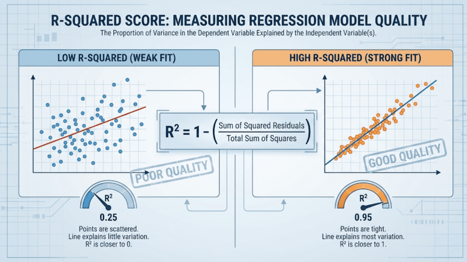
The R-squared score (R²), also called the coefficient of determination, measures how much of the variance in the target variable is explained by a regression model. It ranges from 0 to 1 in well-behaved cases, where 1 means the model perfectly predicts every value and 0 means it does no better than simply predicting the mean of the target. Unlike MAE or RMSE, R² is unit-free and scale-independent, making it ideal for comparing models across different datasets.
Introduction
You have trained a regression model to predict house prices. Your RMSE is $32,500. Is that good or bad?
The honest answer is: it depends entirely on context. An RMSE of $32,500 is excellent if you’re predicting mansions worth $5 million. It is terrible if you’re predicting starter homes worth $150,000. Without knowing the scale and variability of your target, absolute error metrics like RMSE and MAE cannot tell you how well your model is really doing relative to what’s achievable.
This is the problem that R-squared (R²) solves.
R² is a normalized, dimensionless measure of model quality that answers a fundamentally different question than MAE or RMSE: “How much better does my model predict than the simplest possible baseline?” That baseline is the mean of the target variable — the naïve prediction that ignores all features entirely. R² tells you what fraction of the target’s natural variability your model succeeds in explaining.
In this article we’ll build R² from first principles, explore its geometric and statistical meaning, implement it in Python, understand its important limitations, meet its improved cousin Adjusted R², and develop a complete framework for using R² correctly in regression evaluation.
Building Intuition: Variance as a Baseline
Before we define R², we need to understand what we’re comparing against.
The Naïve Baseline: Predicting the Mean
Imagine your dataset contains house prices: $180k, $220k, $195k, $310k, $250k. You are asked to predict each price without using any features at all — no square footage, no location, no number of rooms, nothing.
The best single number you could predict for every house is the mean price: $231k. This minimizes the sum of squared errors when you have no other information. Any model that uses features should do better than this baseline.
Total Variance: How Spread Out Is the Target?
The Total Sum of Squares (SS_tot) measures how much the target values vary around their mean:
Where ȳ (y-bar) is the mean of all actual target values. SS_tot captures the total amount of variability in the data that any model could potentially explain. If all house prices were identical, SS_tot = 0 and the problem would be trivially solved.
Residual Variance: How Much Your Model Fails to Explain
The Residual Sum of Squares (SS_res) — also called the Sum of Squared Errors (SSE) — measures how much variability remains after your model makes its predictions:
This is the variability your model could not explain. If SS_res = 0, every prediction is perfect. If SS_res = SS_tot, your model explains nothing — it performs exactly as poorly as the mean baseline.
The R-squared Formula
With these components in place, R² has an elegant definition:
Interpreting the Formula
The ratio SS_res / SS_tot is the fraction of variance not explained by the model. Subtracting it from 1 gives the fraction of variance that is explained.
- If SS_res = 0 (perfect predictions): R² = 1 − 0 = 1.0 (perfect)
- If SS_res = SS_tot (model as bad as the mean): R² = 1 − 1 = 0.0 (no explanatory power)
- If SS_res > SS_tot (model worse than the mean): R² < 0 (negative R²!)
The third case is surprising to many beginners. R² can be negative. This happens when your model is so badly miscalibrated that it performs worse than simply predicting the mean for every sample. A model that achieves negative R² is actively harmful.
An Alternative Derivation
R² can also be derived from the ratio of explained variance to total variance:
This formulation makes the “fraction of explained variance” interpretation even more direct.
A Worked Example
Let’s compute R² manually on our five apartment prices:
| Sample | Actual (y) | Predicted (ŷ) | Residual (y – ŷ) | Residual² | (y – ȳ)² |
|---|---|---|---|---|---|
| 1 | $1,200 | $1,150 | $50 | 2,500 | 376,900 |
| 2 | $2,500 | $2,600 | -$100 | 10,000 | 1,014,400 |
| 3 | $800 | $780 | $20 | 400 | 984,100 |
| 4 | $3,200 | $3,100 | $100 | 10,000 | 3,276,900 |
| 5 | $1,500 | $1,580 | -$80 | 6,400 | 12,100 |
Mean (ȳ) = (1200 + 2500 + 800 + 3200 + 1500) / 5 = $1,840
An R² of 0.9948 means the model explains 99.48% of the variance in apartment prices. Only 0.52% of the variance remains unexplained. That’s an excellent result.
Geometric Interpretation of R²
The geometric picture of R² is illuminating. Imagine plotting actual vs predicted values on a scatter plot:
- A perfect model (R² = 1.0) produces all points exactly on the diagonal line y = ŷ
- A mean-predicting baseline (R² = 0.0) produces a horizontal band — all predictions equal to ȳ regardless of x
- A good model (R² = 0.85) produces points that cluster tightly around the diagonal with modest scatter
The tighter the points cluster around the diagonal, the higher the R². The horizontal spread of points off the diagonal represents unexplained residual variance.
For simple linear regression with one feature, R² equals the square of Pearson’s correlation coefficient r:
This is where the name “R-squared” originates. In multivariate regression, R² is no longer simply the square of a single correlation, but the name and symbol persist.
Python Implementation: From Scratch to Scikit-learn
Manual Computation
import numpy as np
import matplotlib.pyplot as plt
import matplotlib.gridspec as gridspec

def compute_r_squared(y_true, y_pred):
    """
    Compute R-squared (coefficient of determination) from scratch.

    Args:
        y_true: Array of actual target values
        y_pred: Array of predicted values

    Returns:
        Dictionary with R², SS_res, SS_tot, and all components
    """
    y_true = np.array(y_true, dtype=float)
    y_pred = np.array(y_pred, dtype=float)

    y_mean = np.mean(y_true)

    # Sum of squared residuals (unexplained variance)
    ss_res = np.sum((y_true - y_pred) ** 2)

    # Total sum of squares (total variance)
    ss_tot = np.sum((y_true - y_mean) ** 2)

    # Explained sum of squares (variance explained by model)
    ss_exp = ss_tot - ss_res

    # R-squared
    r2 = 1 - (ss_res / ss_tot) if ss_tot > 0 else 0.0

    return {
        "R_squared":  r2,
        "SS_res":     ss_res,
        "SS_tot":     ss_tot,
        "SS_exp":     ss_exp,
        "y_mean":     y_mean,
        "pct_explained": r2 * 100,
        "pct_unexplained": (1 - r2) * 100
    }


# ----- Example 1: Apartment rent (our earlier example) -----
y_actual = np.array([1200, 2500, 800, 3200, 1500], dtype=float)
y_pred   = np.array([1150, 2600, 780, 3100, 1580], dtype=float)

result = compute_r_squared(y_actual, y_pred)
print("=== Apartment Rent Prediction ===\n")
print(f"  Mean of actuals (ȳ): ${result['y_mean']:.0f}")
print(f"  SS_res (unexplained): {result['SS_res']:,.0f}")
print(f"  SS_tot (total):       {result['SS_tot']:,.0f}")
print(f"  SS_exp (explained):   {result['SS_exp']:,.0f}")
print(f"\n  R² = {result['R_squared']:.4f}")
print(f"  Model explains {result['pct_explained']:.2f}% of variance")
print(f"  {result['pct_unexplained']:.2f}% of variance is unexplained")


# ----- Example 2: Three models at different quality levels -----
print("\n=== Comparing Three Models ===\n")
y_true_ex = np.array([10, 20, 30, 40, 50, 60, 70, 80, 90, 100], dtype=float)

models_comparison = {
    "Perfect model":        np.array([10, 20, 30, 40, 50, 60, 70, 80, 90, 100]),
    "Good model":           np.array([12, 18, 32, 38, 52, 58, 73, 77, 92, 98]),
    "Mean baseline":        np.full(10, y_true_ex.mean()),
    "Terrible model":       np.array([90, 80, 70, 60, 50, 40, 30, 20, 10, 5]),  # Near-opposite
}

print(f"{'Model':<25} | {'R²':>8} | {'Interpretation'}")
print("-" * 65)

for name, y_pred_m in models_comparison.items():
    r = compute_r_squared(y_true_ex, y_pred_m)
    r2_val = r['R_squared']

    if r2_val >= 0.99:
        interp = "Perfect — predicts every value exactly"
    elif r2_val >= 0.90:
        interp = "Excellent — explains >90% of variance"
    elif r2_val >= 0.70:
        interp = "Good — explains majority of variance"
    elif r2_val >= 0.50:
        interp = "Moderate — explains more than half"
    elif r2_val > 0.0:
        interp = "Weak — explains some variance"
    elif r2_val == 0.0:
        interp = "No better than predicting the mean"
    else:
        interp = f"Negative! Worse than the mean baseline"

print(f"{name:<25} | {r2_val:>8.4f} | {interp}")Scikit-learn Implementation
from sklearn.metrics import r2_score
from sklearn.datasets import fetch_california_housing
from sklearn.linear_model import LinearRegression, Ridge, Lasso
from sklearn.ensemble import RandomForestRegressor, GradientBoostingRegressor
from sklearn.model_selection import train_test_split, cross_val_score
from sklearn.preprocessing import StandardScaler, PolynomialFeatures
from sklearn.pipeline import Pipeline
import numpy as np

# Load California housing dataset
housing = fetch_california_housing()
X, y = housing.data, housing.target
feature_names = housing.feature_names

X_train, X_test, y_train, y_test = train_test_split(
    X, y, test_size=0.2, random_state=42
)

# Scale features for linear models
scaler = StandardScaler()
X_train_s = scaler.fit_transform(X_train)
X_test_s  = scaler.transform(X_test)

# Train and evaluate multiple models
models = {
    "Linear Regression":       (LinearRegression(), True),
    "Ridge Regression":        (Ridge(alpha=1.0), True),
    "Lasso Regression":        (Lasso(alpha=0.01, max_iter=5000), True),
    "Polynomial (degree=2)":   (Pipeline([
                                   ('poly', PolynomialFeatures(degree=2, include_bias=False)),
                                   ('ridge', Ridge(alpha=1.0))
                                ]), True),
    "Random Forest":           (RandomForestRegressor(200, random_state=42, n_jobs=-1), False),
    "Gradient Boosting":       (GradientBoostingRegressor(200, random_state=42), False),
}

print("=== California Housing: R² Score Comparison ===\n")
print(f"{'Model':<28} | {'Train R²':>9} | {'Test R²':>8} | {'Overfit Gap':>12}")
print("-" * 65)

results = {}
for name, (model, needs_scaling) in models.items():
    X_tr = X_train_s if needs_scaling else X_train
    X_te = X_test_s  if needs_scaling else X_test

    model.fit(X_tr, y_train)

    train_r2 = r2_score(y_train, model.predict(X_tr))
    test_r2  = r2_score(y_test,  model.predict(X_te))
    gap = train_r2 - test_r2

    results[name] = {"train_r2": train_r2, "test_r2": test_r2, "gap": gap}
    flag = " ← OVERFIT" if gap > 0.10 else ""
    print(f"{name:<28} | {train_r2:>9.4f} | {test_r2:>8.4f} | {gap:>12.4f}{flag}")

print("\nNote: Large gap between train R² and test R² indicates overfitting.")Cross-Validated R²
from sklearn.model_selection import StratifiedKFold, KFold, cross_val_score

# Use KFold for regression (not StratifiedKFold, which is for classification)
kf = KFold(n_splits=5, shuffle=True, random_state=42)

print("\n=== 5-Fold Cross-Validated R² ===\n")
print(f"{'Model':<28} | {'Mean R²':>8} | {'Std Dev':>8} | {'Min':>7} | {'Max':>7}")
print("-" * 68)

for name, (model, needs_scaling) in models.items():
    X_data = X_train_s if needs_scaling else X_train

    cv_scores = cross_val_score(model, X_data, y_train, cv=kf, scoring='r2')

    print(f"{name:<28} | {cv_scores.mean():>8.4f} | {cv_scores.std():>8.4f} | "
          f"{cv_scores.min():>7.4f} | {cv_scores.max():>7.4f}")

print("\nCross-validated R² is more reliable than single train/test split.")Visualizing R²: What the Numbers Mean
Concrete visualizations build intuition for what different R² values actually look like.
import numpy as np
import matplotlib.pyplot as plt

def visualize_r2_levels():
    """
    Generate scatter plots showing what R² looks like at different levels.
    Creates six panels: R² ≈ 1.0, 0.9, 0.7, 0.5, 0.2, negative.
    """
    np.random.seed(42)
    n = 200
    x = np.linspace(0, 10, n)

    # True linear relationship
    y_true_signal = 2 * x + 5

    # Add different levels of noise to achieve different R² values
    noise_levels = {
        "R² ≈ 1.00": 0.1,
        "R² ≈ 0.90": 1.5,
        "R² ≈ 0.70": 3.0,
        "R² ≈ 0.50": 5.0,
        "R² ≈ 0.20": 10.0,
        "R² < 0 (negative)": None  # Random predictions
    }

    fig, axes = plt.subplots(2, 3, figsize=(15, 9))
    axes = axes.flatten()

    for ax, (title, noise) in zip(axes, noise_levels.items()):
        if noise is None:
            # Predictions that are completely random / anti-correlated
            y_obs  = y_true_signal + np.random.normal(0, 3, n)
            y_pred = np.random.uniform(0, 10, n)  # Random predictions
        else:
            y_obs  = y_true_signal + np.random.normal(0, noise, n)
            # Linear regression predictions (approximate)
            from sklearn.linear_model import LinearRegression
            lr = LinearRegression()
            lr.fit(x.reshape(-1, 1), y_obs)
            y_pred = lr.predict(x.reshape(-1, 1))

        # Compute actual R²
        actual_r2 = r2_score(y_obs, y_pred)

        ax.scatter(y_obs, y_pred, alpha=0.3, s=12, color='steelblue')

        # Perfect prediction line
        all_vals = np.concatenate([y_obs, y_pred])
        min_val, max_val = all_vals.min(), all_vals.max()
        ax.plot([min_val, max_val], [min_val, max_val], 'r--', lw=2, label='Perfect')

        # Mean baseline (horizontal line)
        ax.axhline(y=y_obs.mean(), color='orange', linestyle=':', lw=1.5,
                   label=f'Mean={y_obs.mean():.1f}')

        ax.set_xlabel("Actual Values", fontsize=10)
        ax.set_ylabel("Predicted Values", fontsize=10)
        ax.set_title(f"{title}\n(Actual R² = {actual_r2:.3f})",
                     fontsize=11, fontweight='bold')
        ax.legend(fontsize=8)
        ax.grid(True, alpha=0.3)

    plt.suptitle("What Different R² Values Look Like", fontsize=14, fontweight='bold', y=1.01)
    plt.tight_layout()
    plt.savefig("r2_visualization_levels.png", dpi=150, bbox_inches='tight')
    plt.show()
    print("Saved: r2_visualization_levels.png")

visualize_r2_levels()The Variance Decomposition: A Deeper Look
The R² score rests on a clean mathematical decomposition of total variance. In ordinary least squares (OLS) linear regression, the total sum of squares perfectly decomposes into explained and unexplained components:
This is called the variance decomposition theorem (or ANOVA decomposition). It is guaranteed to hold for OLS linear regression with an intercept term. For other model types (neural networks, decision trees, non-linear models), this exact decomposition may not hold, though R² remains a useful metric in practice.
The three components have intuitive interpretations:
SS_tot: How much do the actual target values vary? This is a property of the data, not your model.
SS_exp: How much of that variation does your model capture? This is the “signal” your model learned.
SS_res: How much variation remains in the errors? This is the “noise” your model couldn’t capture.
import numpy as np
from sklearn.linear_model import LinearRegression
from sklearn.datasets import fetch_california_housing
from sklearn.model_selection import train_test_split
from sklearn.metrics import r2_score

# Demonstrate variance decomposition
housing = fetch_california_housing()
X, y = housing.data[:, :2], housing.target  # Use just 2 features for simplicity

X_train, X_test, y_train, y_test = train_test_split(X, y, test_size=0.2, random_state=42)

lr = LinearRegression()
lr.fit(X_train, y_train)
y_pred = lr.predict(X_test)

y_mean = np.mean(y_test)
ss_tot = np.sum((y_test - y_mean) ** 2)
ss_res = np.sum((y_test - y_pred) ** 2)
ss_exp = np.sum((y_pred - y_mean) ** 2)

print("=== Variance Decomposition ===\n")
print(f"  SS_tot (total variance):       {ss_tot:>12,.2f}")
print(f"  SS_exp (explained by model):   {ss_exp:>12,.2f}")
print(f"  SS_res (residual/unexplained): {ss_res:>12,.2f}")
print(f"  SS_exp + SS_res:               {ss_exp + ss_res:>12,.2f}")
print(f"\n  Decomposition holds: {np.isclose(ss_tot, ss_exp + ss_res, rtol=0.001)}")
print(f"\n  R² = SS_exp/SS_tot = {ss_exp/ss_tot:.4f}")
print(f"  R² = 1 - SS_res/SS_tot = {1 - ss_res/ss_tot:.4f}")
print(f" Sklearn r2_score: {r2_score(y_test, y_pred):.4f}")R-squared and Pearson Correlation
For simple linear regression (one feature, one target), R² is exactly the square of Pearson’s correlation coefficient r:
This connection is important for several reasons. First, it shows that R² is symmetric — it doesn’t matter which variable you call “input” and which you call “output” in a simple linear model. Second, it gives R² a direct interpretation in terms of linear association strength.
import numpy as np
from scipy.stats import pearsonr
from sklearn.linear_model import LinearRegression
from sklearn.metrics import r2_score

np.random.seed(42)
n = 200
x = np.random.uniform(0, 10, n)

# Different correlation strengths
correlations = [0.95, 0.80, 0.60, 0.30]

print("=== R² = r² for Simple Linear Regression ===\n")
print(f"{'Pearson r':>10} | {'r² (expected R²)':>17} | {'Actual R²':>10} | Match?")
print("-" * 55)

for target_r in correlations:
    # Generate y with specific correlation to x
    noise_scale = np.sqrt((1 - target_r**2) / target_r**2) if target_r < 1 else 0
    y = x + np.random.normal(0, noise_scale * x.std(), n)

    # Actual Pearson correlation
    r, _ = pearsonr(x, y)

    # Linear regression R²
    lr = LinearRegression()
    lr.fit(x.reshape(-1, 1), y)
    y_pred = lr.predict(x.reshape(-1, 1))
    actual_r2 = r2_score(y, y_pred)

    expected_r2 = r**2
    match = "✓" if np.isclose(expected_r2, actual_r2, atol=0.001) else "✗"

    print(f"{r:>10.4f} | {expected_r2:>17.4f} | {actual_r2:>10.4f} | {match}")

print("\nNote: This equality holds ONLY for simple linear regression.")
print("For multiple regression or non-linear models, use R² directly.")Critical Limitations of R-squared
R² is powerful but has several important limitations that every practitioner must know. These are the situations where R² can mislead you.
Limitation 1: R² Always Increases With More Features
This is the most dangerous property of R². Adding any new feature to a linear regression model — even a completely random, useless one — will never decrease R² on the training data. It will either stay the same or slightly increase, because more parameters give the model more flexibility to fit noise.
import numpy as np
from sklearn.linear_model import LinearRegression
from sklearn.metrics import r2_score

np.random.seed(42)
n = 100

# True relationship: y depends only on x1
x1 = np.random.normal(0, 1, n)
y  = 3 * x1 + np.random.normal(0, 1, n)

print("=== R² Increases When Adding Random Features (Training Data) ===\n")
print(f"{'Num Features':>13} | {'Train R²':>9} | {'Note'}")
print("-" * 60)

for n_random_features in [0, 1, 5, 10, 20, 50, 98]:
    # Build feature matrix: x1 + n_random_features completely random columns
    random_features = np.random.normal(0, 1, (n, n_random_features))
    X_mat = np.column_stack([x1] + [random_features]) if n_random_features > 0 else x1.reshape(-1, 1)

    lr = LinearRegression()
    lr.fit(X_mat, y)
    train_r2 = r2_score(y, lr.predict(X_mat))

    note = "← Only real feature" if n_random_features == 0 else \
           f"← {n_random_features} pure noise features added"

    print(f"{1 + n_random_features:>13} | {train_r2:>9.4f} | {note}")

print("\nWith 99 features for 100 samples, R² approaches 1.0 on training data!")
print("This is pure overfitting — test R² would be near 0 or negative.")This is why we always report R² on the test set or use cross-validation, not the training set.
Limitation 2: R² Does Not Validate Your Model Assumptions
Anscombe’s Quartet is a famous collection of four datasets, each with nearly identical R² scores (~0.67), means, and variances — yet they have completely different relationships and underlying structures.
import numpy as np
import matplotlib.pyplot as plt
from sklearn.linear_model import LinearRegression
from sklearn.metrics import r2_score

# Anscombe's Quartet — four datasets with identical statistics
anscombe = {
    "Dataset I\n(Linear, appropriate)": {
        "x": [10, 8, 13, 9, 11, 14, 6, 4, 12, 7, 5],
        "y": [8.04, 6.95, 7.58, 8.81, 8.33, 9.96, 7.24, 4.26, 10.84, 4.82, 5.68]
    },
    "Dataset II\n(Curved, linear is wrong)": {
        "x": [10, 8, 13, 9, 11, 14, 6, 4, 12, 7, 5],
        "y": [9.14, 8.14, 8.74, 8.77, 9.26, 8.10, 6.13, 3.10, 9.13, 7.26, 4.74]
    },
    "Dataset III\n(Outlier pulls fit)": {
        "x": [10, 8, 13, 9, 11, 14, 6, 4, 12, 7, 5],
        "y": [7.46, 6.77, 12.74, 7.11, 7.81, 8.84, 6.08, 5.39, 8.15, 6.42, 5.73]
    },
    "Dataset IV\n(Leverage point)": {
        "x": [8, 8, 8, 8, 8, 8, 8, 19, 8, 8, 8],
        "y": [6.58, 5.76, 7.71, 8.84, 8.47, 7.04, 5.25, 12.50, 5.56, 7.91, 6.89]
    },
}

fig, axes = plt.subplots(2, 2, figsize=(13, 10))
axes = axes.flatten()

for ax, (title, data) in zip(axes, anscombe.items()):
    x_arr = np.array(data["x"], dtype=float)
    y_arr = np.array(data["y"], dtype=float)

    lr = LinearRegression()
    lr.fit(x_arr.reshape(-1, 1), y_arr)
    y_fit = lr.predict(x_arr.reshape(-1, 1))
    r2 = r2_score(y_arr, y_fit)

    ax.scatter(x_arr, y_arr, color='steelblue', s=80, zorder=5)
    x_line = np.linspace(x_arr.min() - 1, x_arr.max() + 1, 100)
    ax.plot(x_line, lr.predict(x_line.reshape(-1, 1)), 'r-', lw=2, label=f'R²={r2:.3f}')
    ax.set_title(title, fontsize=11, fontweight='bold')
    ax.set_xlabel("x", fontsize=10)
    ax.set_ylabel("y", fontsize=10)
    ax.legend(fontsize=11)
    ax.grid(True, alpha=0.3)

plt.suptitle("Anscombe's Quartet: Same R² ≈ 0.67, Completely Different Relationships",
             fontsize=13, fontweight='bold', y=1.01)
plt.tight_layout()
plt.savefig("anscombe_quartet.png", dpi=150, bbox_inches='tight')
plt.show()
print("Saved: anscombe_quartet.png")
print("\nKey lesson: Always plot your data and residuals — never rely on R² alone!")Limitation 3: R² Is Affected by the Range of the Target Variable
Restricting your data to a narrower range of the target variable automatically decreases R². Suppose you have a model that predicts house prices well across the full range $100k–$2M. If you evaluate it only on homes in the $300k–$400k range, the total variance (SS_tot) is much smaller, and the model’s R² will appear lower — even though the model hasn’t changed.
This is why you should be careful comparing R² scores across different datasets or different subsets of the same dataset.
Limitation 4: R² Cannot Compare Models Across Different Targets
A model predicting stock prices with R² = 0.60 is not necessarily better than a model predicting energy consumption with R² = 0.75. R² is meaningful only relative to the baseline variance in the specific target variable you are modeling.
Limitation 5: High R² Does Not Mean Good Predictions
A model can achieve high R² while still producing absolute errors that are too large to be useful for a particular application. If you need predictions within ±$5,000 but your model has MAE = $50,000, an R² of 0.90 is irrelevant to whether the model is fit for purpose.
Adjusted R-squared: Correcting for Feature Count
Because R² always increases when you add features, it cannot be used to compare models with different numbers of features on training data. Adjusted R² corrects for this by penalizing model complexity.
Formula
Where:
- n = number of samples in the dataset
- k = number of predictor features (not counting the intercept)
- R² = the ordinary R-squared
The fraction (n-1)/(n-k-1) is always ≥ 1, so Adjusted R² ≤ R². When you add a feature that genuinely improves the model, R² increases enough to outweigh the penalty and Adjusted R² also increases. When you add a useless feature, R² barely increases but the penalty grows, causing Adjusted R² to decrease.
Key Properties of Adjusted R²
- Adjusted R² can be negative even when R² is positive
- For a single feature model, Adjusted R² is close to R²
- Adjusted R² is appropriate for comparing models with different numbers of features on the same training data
- It is still better to use test-set R² or cross-validated R² for model selection
import numpy as np
from sklearn.linear_model import LinearRegression
from sklearn.metrics import r2_score

def adjusted_r2(r2, n, k):
    """
    Compute Adjusted R² from R², number of samples, and number of features.

    Args:
        r2: Ordinary R-squared
        n:  Number of samples
        k:  Number of predictor features

    Returns:
        Adjusted R²
    """
    if n <= k + 1:
        raise ValueError("n must be greater than k + 1")
    return 1 - (1 - r2) * (n - 1) / (n - k - 1)


# Demonstrate how Adjusted R² penalizes unnecessary features
np.random.seed(42)
n = 100
x1 = np.random.normal(0, 1, n)
y  = 3 * x1 + np.random.normal(0, 1, n)

print("=== Adjusted R² vs R² as Features Are Added ===\n")
print(f"{'Num Features':>13} | {'Train R²':>9} | {'Adj R²':>8} | {'Adj R² change':>14}")
print("-" * 55)

prev_adj_r2 = None
for n_features in [1, 2, 5, 10, 20, 50]:
    random_cols = np.random.normal(0, 1, (n, n_features - 1))
    X_mat = np.column_stack([x1.reshape(-1, 1), random_cols]) if n_features > 1 else x1.reshape(-1, 1)

    lr = LinearRegression()
    lr.fit(X_mat, y)
    train_r2 = r2_score(y, lr.predict(X_mat))
    adj_r2   = adjusted_r2(train_r2, n, n_features)

    change_str = ""
    if prev_adj_r2 is not None:
        delta = adj_r2 - prev_adj_r2
        change_str = f"{delta:>+.4f} {'↑' if delta > 0 else '↓'}"

    print(f"{n_features:>13} | {train_r2:>9.4f} | {adj_r2:>8.4f} | {change_str}")
    prev_adj_r2 = adj_r2

print("\nR² keeps climbing; Adjusted R² falls when useless features are added.")When to Use Adjusted R²
Adjusted R² is most useful in classical statistical modeling (linear regression, GLMs) when comparing models built on the same training data with different feature sets. In machine learning contexts, cross-validated R² on held-out data is generally preferred for model selection because it directly estimates out-of-sample performance.
Residual Analysis: What R² Doesn’t Tell You
A high R² score is a necessary but not sufficient condition for a good model. You must always analyze the residuals — the individual prediction errors — to verify that the model’s assumptions are being met.
What Good Residuals Look Like
For a well-specified regression model, residuals should be:
- Centered around zero — no systematic over- or under-prediction
- Homoscedastic — constant variance across all predicted values (no funnel shape)
- Uncorrelated with predictions — no remaining pattern to be captured
- Approximately normally distributed — if using methods that rely on this assumption
import numpy as np
import matplotlib.pyplot as plt
import matplotlib.gridspec as gridspec
from sklearn.linear_model import LinearRegression
from sklearn.datasets import fetch_california_housing
from sklearn.model_selection import train_test_split
from sklearn.metrics import r2_score
from scipy import stats

def residual_analysis_plot(y_true, y_pred, model_name="Model"):
    """
    Four-panel residual analysis:
    1. Residuals vs Predicted (tests homoscedasticity)
    2. Q-Q plot (tests normality of residuals)
    3. Residuals histogram
    4. Actual vs Predicted
    """
    residuals = y_true - y_pred

    fig = plt.figure(figsize=(15, 10))
    gs  = gridspec.GridSpec(2, 2, figure=fig, hspace=0.4, wspace=0.35)

    # ---- Panel 1: Residuals vs Predicted ----
    ax1 = fig.add_subplot(gs[0, 0])
    ax1.scatter(y_pred, residuals, alpha=0.3, s=10, color='steelblue')
    ax1.axhline(y=0, color='red', linestyle='--', lw=2)
    ax1.set_xlabel("Predicted Values", fontsize=11)
    ax1.set_ylabel("Residuals", fontsize=11)
    ax1.set_title("Residuals vs Predicted\n(Should show random scatter around 0)",
                  fontsize=11, fontweight='bold')
    ax1.grid(True, alpha=0.3)

    # ---- Panel 2: Q-Q Plot ----
    ax2 = fig.add_subplot(gs[0, 1])
    (osm, osr), (slope, intercept, r_val) = stats.probplot(residuals, dist="norm")
    ax2.scatter(osm, osr, alpha=0.3, s=10, color='coral')
    ax2.plot(osm, slope * np.array(osm) + intercept, 'k-', lw=2, label='Normal line')
    ax2.set_xlabel("Theoretical Quantiles", fontsize=11)
    ax2.set_ylabel("Sample Quantiles", fontsize=11)
    ax2.set_title("Q-Q Plot of Residuals\n(Should follow the straight line)",
                  fontsize=11, fontweight='bold')
    ax2.legend(fontsize=10)
    ax2.grid(True, alpha=0.3)

    # ---- Panel 3: Residuals Histogram ----
    ax3 = fig.add_subplot(gs[1, 0])
    ax3.hist(residuals, bins=50, edgecolor='white', color='mediumseagreen', alpha=0.8)
    ax3.axvline(x=0, color='red', linestyle='--', lw=2)
    ax3.axvline(x=residuals.mean(), color='blue', linestyle='-', lw=2,
                label=f'Mean={residuals.mean():.3f}')
    ax3.set_xlabel("Residual Value", fontsize=11)
    ax3.set_ylabel("Frequency", fontsize=11)
    ax3.set_title("Residuals Distribution\n(Should be bell-shaped, centered at 0)",
                  fontsize=11, fontweight='bold')
    ax3.legend(fontsize=10)
    ax3.grid(True, alpha=0.3)

    # ---- Panel 4: Actual vs Predicted ----
    ax4 = fig.add_subplot(gs[1, 1])
    ax4.scatter(y_true, y_pred, alpha=0.3, s=10, color='mediumpurple')
    min_val = min(y_true.min(), y_pred.min())
    max_val = max(y_true.max(), y_pred.max())
    ax4.plot([min_val, max_val], [min_val, max_val], 'r--', lw=2, label='Perfect prediction')

    r2 = r2_score(y_true, y_pred)
    ax4.set_xlabel("Actual Values", fontsize=11)
    ax4.set_ylabel("Predicted Values", fontsize=11)
    ax4.set_title(f"Actual vs Predicted\n(R² = {r2:.4f})",
                  fontsize=11, fontweight='bold')
    ax4.legend(fontsize=10)
    ax4.grid(True, alpha=0.3)

    plt.suptitle(f"Residual Analysis: {model_name}", fontsize=14, fontweight='bold', y=1.02)
    plt.savefig("residual_analysis.png", dpi=150, bbox_inches='tight')
    plt.show()

    # Summary statistics
    print(f"\n=== Residual Summary: {model_name} ===")
    print(f"  R²:               {r2:.4f}")
    print(f"  Mean residual:    {residuals.mean():.4f}  (near 0 is good)")
    print(f"  Std of residuals: {residuals.std():.4f}")
    print(f"  Skewness:         {stats.skew(residuals):.4f}  (near 0 is good)")
    print(f"  Kurtosis:         {stats.kurtosis(residuals):.4f}  (near 0 for normal)")
    print("Saved: residual_analysis.png")


# Apply residual analysis to California housing
housing = fetch_california_housing()
X, y = housing.data, housing.target
X_train, X_test, y_train, y_test = train_test_split(X, y, test_size=0.2, random_state=42)

scaler = StandardScaler()
X_train_s = scaler.fit_transform(X_train)
X_test_s  = scaler.transform(X_test)

lr = LinearRegression()
lr.fit(X_train_s, y_train)
y_pred = lr.predict(X_test_s)

residual_analysis_plot(y_test, y_pred, "Linear Regression (California Housing)")When Is R² High Enough? Domain-Specific Benchmarks
One of the most common questions from beginners is: “What is a good R² score?” The answer is deeply domain-dependent.
| Domain | Typical R² Range | Notes |
|---|---|---|
| Physical sciences (e.g., Hooke’s Law) | 0.99 – 1.00 | Deterministic relationships; near-perfect is expected |
| Engineering (structural loads, materials) | 0.95 – 0.99 | Tight physical constraints |
| Controlled laboratory experiments | 0.90 – 0.99 | Low noise, controlled variables |
| Medical measurements (e.g., blood markers) | 0.70 – 0.90 | Biological variability present |
| Economic / financial modeling | 0.30 – 0.70 | Markets are inherently noisy and unpredictable |
| Social science / psychology surveys | 0.10 – 0.50 | Human behavior is complex and variable |
| Stock price forecasting (next-day) | 0.01 – 0.05 | Near-random; even 0.05 can be profitable |
| Weather prediction (7-day ahead) | 0.20 – 0.50 | Chaotic system; moderate R² is acceptable |
These ranges are rough guidelines. An R² of 0.40 in stock price prediction might represent an extraordinary achievement; an R² of 0.40 in a physics experiment would be considered a failure of the experimental setup.
The key principle: compare your R² to domain benchmarks and to simpler baselines, not to an abstract ideal.
R² for Non-Linear Models: A Nuance
R² is most naturally interpreted in the context of linear regression. For non-linear models (neural networks, tree ensembles, SVMs), R² is still mathematically computable and meaningful, but some properties change:
- The variance decomposition SS_tot = SS_exp + SS_res may not hold exactly
- The connection to Pearson’s r is lost
- R² can still be negative if the non-linear model performs very poorly
In practice, R² is widely used to evaluate all types of regression models and remains interpretable as “proportion of explained variance” regardless of model type.
from sklearn.metrics import r2_score
from sklearn.ensemble import GradientBoostingRegressor
from sklearn.linear_model import LinearRegression
import numpy as np

# Non-linear relationship: y = sin(x) + noise
np.random.seed(42)
n = 300
x = np.linspace(0, 4 * np.pi, n)
y = np.sin(x) + 0.3 * np.random.normal(0, 1, n)

X = x.reshape(-1, 1)
X_train, X_test, y_train, y_test = train_test_split(X, y, test_size=0.2, random_state=42)

# Linear model (wrong functional form)
lr = LinearRegression()
lr.fit(X_train, y_train)
y_pred_lr = lr.predict(X_test)

# Non-linear model (correct functional form)
gbm = GradientBoostingRegressor(n_estimators=300, max_depth=4, random_state=42)
gbm.fit(X_train.ravel().reshape(-1, 1), y_train)
y_pred_gbm = gbm.predict(X_test.ravel().reshape(-1, 1))

print("=== R² for Linear vs Non-linear Model on Sinusoidal Data ===\n")
print(f"Linear Regression R²:   {r2_score(y_test, y_pred_lr):.4f}")
print(f"Gradient Boosting R²:   {r2_score(y_test, y_pred_gbm):.4f}")
print("\nLinear model has low/negative R² because the functional form is wrong.")
print("R² correctly reveals model misspecification.")Complete Evaluation Framework: Combining All Regression Metrics
In practice, never rely on a single metric. Use a combination of metrics that together give a complete picture.
import numpy as np
from sklearn.metrics import r2_score, mean_absolute_error, mean_squared_error
from sklearn.datasets import fetch_california_housing
from sklearn.ensemble import GradientBoostingRegressor, RandomForestRegressor
from sklearn.linear_model import LinearRegression
from sklearn.model_selection import KFold, cross_validate
from sklearn.preprocessing import StandardScaler
import warnings
warnings.filterwarnings('ignore')

def comprehensive_regression_evaluation(model, X_train, X_test, y_train, y_test,
                                          model_name="Model", n_cv_folds=5):
    """
    Complete regression model evaluation using all key metrics.

    Reports:
    - Test-set R², MAE, RMSE, MAPE
    - Training R² for overfitting check
    - Cross-validated R² with confidence interval
    - Adjusted R²
    - Residual diagnostics
    """
    from sklearn.preprocessing import StandardScaler

    # Fit and predict
    model.fit(X_train, y_train)
    y_pred_train = model.predict(X_train)
    y_pred_test  = model.predict(X_test)

    # Core metrics
    train_r2 = r2_score(y_train, y_pred_train)
    test_r2  = r2_score(y_test, y_pred_test)
    test_mae  = mean_absolute_error(y_test, y_pred_test)
    test_rmse = np.sqrt(mean_squared_error(y_test, y_pred_test))
    test_mape = np.mean(np.abs((y_test - y_pred_test) / np.clip(y_test, 1e-8, None))) * 100

    # Adjusted R²
    n, k = X_test.shape
    adj_r2 = 1 - (1 - test_r2) * (n - 1) / (n - k - 1)

    # Cross-validated R²
    kf = KFold(n_splits=n_cv_folds, shuffle=True, random_state=42)
    X_all = np.vstack([X_train, X_test])
    y_all = np.concatenate([y_train, y_test])
    cv_results = cross_validate(model, X_all, y_all, cv=kf,
                                 scoring='r2', return_train_score=True)
    cv_r2_mean = cv_results['test_score'].mean()
    cv_r2_std  = cv_results['test_score'].std()

    # Residual statistics
    residuals = y_test - y_pred_test
    residual_mean = residuals.mean()
    residual_std  = residuals.std()
    rmse_mae_ratio = test_rmse / test_mae if test_mae > 0 else float('inf')

    print(f"\n{'='*55}")
    print(f"  {model_name}")
    print(f"{'='*55}")
    print(f"\n  Explained Variance:")
    print(f"    Test R²:          {test_r2:.4f}  ({test_r2*100:.1f}% of variance explained)")
    print(f"    Adjusted R²:      {adj_r2:.4f}")
    print(f"    Train R²:         {train_r2:.4f}  (overfit gap: {train_r2 - test_r2:+.4f})")
    print(f"    CV R²:            {cv_r2_mean:.4f} ± {cv_r2_std:.4f}")

    print(f"\n  Absolute Errors:")
    print(f"    MAE:              {test_mae:.4f}")
    print(f"    RMSE:             {test_rmse:.4f}")
    print(f"    MAPE:             {test_mape:.2f}%")
    print(f"    RMSE/MAE ratio:   {rmse_mae_ratio:.3f}  (1.0=uniform, higher=outliers)")

    print(f"\n  Residual Health:")
    print(f"    Mean residual:    {residual_mean:.4f}  (near 0 = unbiased)")
    print(f"    Residual std:     {residual_std:.4f}")

    # Interpretation flags
    flags = []
    if train_r2 - test_r2 > 0.10:
        flags.append("⚠ Possible overfitting (large train-test R² gap)")
    if test_r2 < 0:
        flags.append("⚠ Negative R² — model worse than mean baseline")
    if rmse_mae_ratio > 2.0:
        flags.append("⚠ High RMSE/MAE ratio — investigate outlier predictions")
    if abs(residual_mean) > 0.01 * y_test.mean():
        flags.append("⚠ Residual mean not near zero — possible bias")

    if flags:
        print(f"\n  Flags:")
        for flag in flags:
            print(f"    {flag}")
    else:
        print(f"\n  ✓ No obvious issues detected")

    return {
        "test_r2": test_r2, "adj_r2": adj_r2, "train_r2": train_r2,
        "cv_r2_mean": cv_r2_mean, "cv_r2_std": cv_r2_std,
        "mae": test_mae, "rmse": test_rmse, "mape": test_mape
    }


# Load data
housing = fetch_california_housing()
X, y = housing.data, housing.target
X_tr, X_te, y_tr, y_te = train_test_split(X, y, test_size=0.2, random_state=42)

scaler = StandardScaler()
X_tr_s = scaler.fit_transform(X_tr)
X_te_s = scaler.transform(X_te)

# Evaluate models
models_eval = [
    ("Linear Regression", LinearRegression(), X_tr_s, X_te_s),
    ("Random Forest",     RandomForestRegressor(200, random_state=42, n_jobs=-1), X_tr, X_te),
    ("Gradient Boosting", GradientBoostingRegressor(200, random_state=42), X_tr, X_te),
]

all_results = {}
for name, model, X_train_m, X_test_m in models_eval:
    all_results[name] = comprehensive_regression_evaluation(
        model, X_train_m, X_test_m, y_tr, y_te, model_name=name
)Summary
R² is arguably the most interpretable single number for characterizing regression model quality. Its core message — “what fraction of the target’s variance does my model explain?” — is immediately understood by technical and non-technical audiences alike.
The formula R² = 1 − (SS_res / SS_tot) tells a clean story: start with all the variance in the target, see how much your model eliminates, and report the fraction eliminated. A perfect model eliminates everything (R² = 1). A model no better than the mean eliminates nothing (R² = 0). A model worse than the mean makes things worse (R² < 0).
However, R² has meaningful limitations that you must respect. It always increases when you add features, making Adjusted R² or cross-validated R² necessary for comparing models of different complexity. It validates nothing about model assumptions, as Anscombe’s Quartet vividly demonstrates — always analyze residuals. It is domain-specific, making it dangerous to apply universal thresholds for what counts as “good.”
Use R² alongside RMSE, MAE, and residual diagnostics for a complete picture of regression model performance. Train-test gap analysis using R² on both sets is one of the clearest and fastest ways to detect overfitting. Cross-validated R² gives the most honest estimate of how well your model will generalize to new data.
Master these complementary metrics and you will be equipped to evaluate any regression model honestly and completely.