Open-loop control is a system where a robot executes commands without checking whether the desired result was actually achieved, while closed-loop control continuously measures the actual outcome and compares it to the desired outcome, using the difference (called error) to automatically correct the robot’s behavior. Closed-loop control—also called feedback control—is the foundation of nearly every precise, reliable robotic system in existence today, from industrial robot arms to self-driving cars.
Introduction
Imagine giving someone directions to your house over the phone. In the first scenario, you say “Drive north for exactly 2.3 miles, then turn left, then drive 0.8 miles.” You hang up and hope for the best—you have no idea if they took a wrong turn, hit traffic, or ended up in the wrong neighborhood. In the second scenario, you stay on the phone with them the entire time: “Okay, you’re at the intersection, now turn left… a bit more… perfect. Now drive forward… slow down, you’re getting close… stop right there.” In the first scenario, you sent a command and had no idea what happened. In the second, you watched the outcome, compared it to your goal, and continuously adjusted your instructions.
This is exactly the difference between open-loop and closed-loop control in robotics. It’s one of the most fundamental concepts in all of control engineering, and understanding it deeply will transform how you think about designing, building, and programming any robotic system. Every motor you’ve ever connected to an Arduino, every servo you’ve positioned, every robot you’ve watched navigate a room—all of them embody one of these two control philosophies. Knowing which to use, when, and why separates the builders who produce reliable robots from those who wonder why their machines never behave quite as expected.
What Is Open-Loop Control?
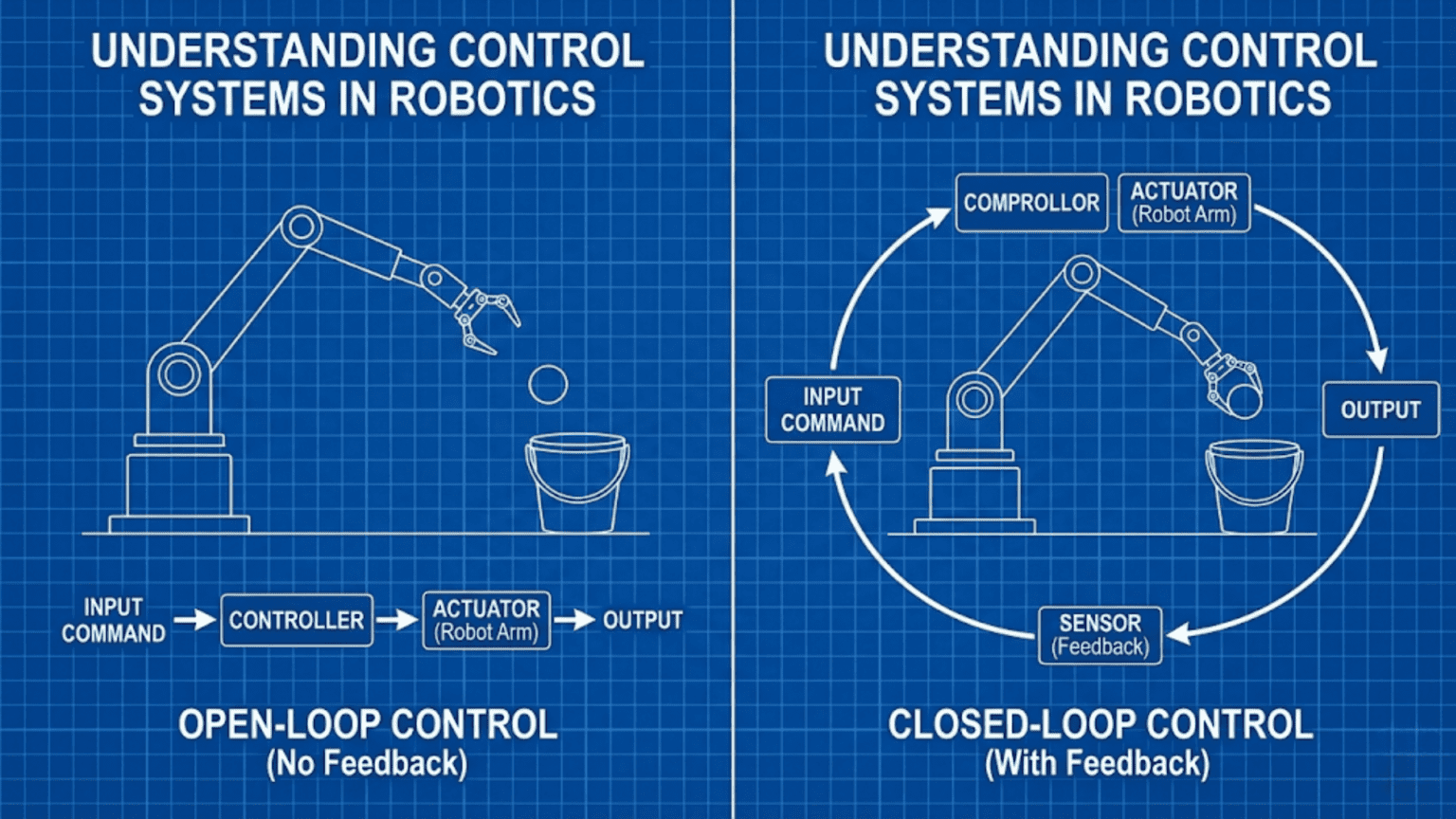
Open-loop control is the simpler of the two approaches. In an open-loop system, the controller sends a command to an actuator—a motor, a heater, a valve, a linear actuator—and the system executes that command without any verification of the result. There is no sensor measuring the outcome, no comparison between what was requested and what actually happened, and no automatic correction mechanism.
The term “open-loop” comes from the idea of signal flow forming an incomplete path. Commands flow from the controller to the actuator to the physical world, but there is no return path bringing information back to the controller. The loop is open—broken—because there is no feedback.
The Structure of an Open-Loop System
An open-loop control system has three basic components:
Reference input: The desired state or output—the goal you want to achieve. This might be “rotate the motor 180 degrees,” “heat the room to 22°C,” or “extend the arm 15 centimeters.”
Controller: The device or algorithm that translates the reference input into a command signal. This might be a microcontroller running code, an analog circuit, or simply a timer.
Plant (or process): The physical system being controlled—the motor, heater, robot arm, or whatever is being driven by the controller’s commands.
The output of the plant (what actually happens in the physical world) has no connection back to the controller. The controller is, in a sense, blind to the results of its own commands.
A Concrete Open-Loop Example
Consider a simple robot that needs to drive forward exactly 50 centimeters. In an open-loop design, you might calculate how long the motors need to run at full power to travel that distance:
// Open-loop distance control
// Assumes robot travels at known constant speed

void setup() {
  pinMode(LEFT_MOTOR_FORWARD, OUTPUT);
  pinMode(RIGHT_MOTOR_FORWARD, OUTPUT);
}

void loop() {
  // Calculate time needed: distance / speed
  // Assume robot moves at 10 cm/s at full power
  // Time needed = 50 cm / 10 cm/s = 5 seconds

  // Drive forward
  digitalWrite(LEFT_MOTOR_FORWARD, HIGH);
  digitalWrite(RIGHT_MOTOR_FORWARD, HIGH);

  delay(5000);  // Run for 5 seconds

  // Stop
  digitalWrite(LEFT_MOTOR_FORWARD, LOW);
  digitalWrite(RIGHT_MOTOR_FORWARD, LOW);

  // Robot assumes it traveled exactly 50 cm
  // No verification whatsoever

  while(true); // Stop after one run
}This code assumes the robot always travels at exactly 10 cm/s. It sends the “drive” command, waits 5 seconds, and sends the “stop” command. It has no idea whether the robot actually traveled 50 centimeters, 47 centimeters, or 53 centimeters. The actual result depends entirely on whether the real-world conditions match the assumed conditions.
When Open-Loop Control Works
Despite its limitations, open-loop control has genuine advantages and real-world applications where it performs reliably. Open-loop systems work well when:
The system is highly consistent and predictable. If you’re controlling a stepper motor in a low-friction environment with no external loads, each pulse reliably produces exactly one step. The physics are so consistent that feedback becomes unnecessary. 3D printers, CNC routers, and many laser cutters use open-loop stepper control with excellent results.
Accuracy requirements are modest. If your robot needs to drive “roughly forward” and exact distance doesn’t matter, open-loop control is perfectly adequate and far simpler to implement.
The disturbances are minimal. If the system never experiences unexpected loads, friction changes, voltage fluctuations, or other disturbing forces, open-loop commands remain accurate.
Cost and simplicity are priorities. Closed-loop control requires sensors, which add cost, weight, complexity, and potential failure points. For inexpensive toys, simple mechanisms, and one-time operations, open-loop control is often the right engineering choice.
The operation time is very short. Errors accumulate over time in open-loop systems. For a quick, brief action, the accumulated error may be negligible.
The Fundamental Weakness of Open-Loop Control
The core problem with open-loop control is that it assumes the real world behaves exactly as modeled. In practice, this assumption always breaks down to some degree. Consider all the things that can cause an open-loop motor control to produce the wrong result:
Battery voltage drops as the battery discharges, causing motors to run slower than calculated. Friction varies depending on the floor surface, wheel wear, and bearing condition. Temperature changes affect motor resistance and torque output. Mechanical wear gradually shifts the relationship between command and output. External loads—a robot arm picking up an unexpectedly heavy object—change the dynamics completely.
An open-loop system has no way to detect or compensate for any of these disturbances. It blindly executes its commands and accepts whatever result the physical world produces.
What Is Closed-Loop Control?
Closed-loop control solves the fundamental limitation of open-loop control by creating a feedback path from the output back to the input. A sensor measures the actual state of the system—the actual position, speed, temperature, or whatever quantity is being controlled—and the controller continuously compares this measured value to the desired value. The difference between desired and actual (the error) drives the controller’s corrective action.
The loop is “closed” because information now flows in a complete circuit: from controller to actuator to physical system to sensor and back to the controller. The system watches what it’s doing and adjusts accordingly.
The Structure of a Closed-Loop System
Closed-loop control adds two critical components to the open-loop structure:
Sensor (feedback element): Measures the actual output of the system. This might be an encoder measuring shaft rotation, a temperature sensor measuring heat, a distance sensor measuring position, or an accelerometer measuring orientation.
Comparator and error calculation: Subtracts the measured output from the desired reference to produce an error signal. This error tells the controller how far off it currently is and in which direction it needs to correct.
The controller then uses this error signal to determine its next command—typically trying to reduce the error toward zero. This process repeats continuously, creating the feedback loop that gives the system its ability to self-correct.
A Concrete Closed-Loop Example
Let’s implement the same 50-centimeter distance challenge using closed-loop control with wheel encoders:
// Closed-loop distance control using wheel encoders

volatile long leftEncoderCount = 0;
volatile long rightEncoderCount = 0;

const int LEFT_ENCODER_PIN = 2;   // Interrupt pin
const int RIGHT_ENCODER_PIN = 3;  // Interrupt pin
const int LEFT_MOTOR_SPEED = 5;   // PWM pin
const int RIGHT_MOTOR_SPEED = 6;  // PWM pin
const int LEFT_MOTOR_DIR = 7;
const int RIGHT_MOTOR_DIR = 8;

const float WHEEL_CIRCUMFERENCE = 20.0;  // cm
const int ENCODER_CPR = 360;             // Counts per revolution

// Interrupt service routines for encoders
void leftEncoderISR() { leftEncoderCount++; }
void rightEncoderISR() { rightEncoderCount++; }

float countsToDistance(long counts) {
  return (counts / (float)ENCODER_CPR) * WHEEL_CIRCUMFERENCE;
}

void driveToDistance(float targetDistance) {
  leftEncoderCount = 0;
  rightEncoderCount = 0;

  int baseSpeed = 150;  // Starting PWM value (0-255)

  while (true) {
    // Calculate actual distance traveled (average of both wheels)
    float leftDistance  = countsToDistance(leftEncoderCount);
    float rightDistance = countsToDistance(rightEncoderCount);
    float actualDistance = (leftDistance + rightDistance) / 2.0;

    // Calculate error (how far we still need to go)
    float error = targetDistance - actualDistance;

    // Are we close enough? (within 0.5 cm)
    if (abs(error) < 0.5) {
      stopMotors();
      Serial.print("Reached target! Actual distance: ");
      Serial.print(actualDistance);
      Serial.println(" cm");
      return;
    }

    // Simple proportional speed reduction as we approach target
    // Full speed until 10 cm away, then slow proportionally
    int speed = baseSpeed;
    if (error < 10.0) {
      speed = (int)(baseSpeed * (error / 10.0));
      speed = max(speed, 60);  // Minimum speed to keep moving
    }

    // Drive forward
    setMotorSpeed(LEFT_MOTOR_SPEED, LEFT_MOTOR_DIR, speed);
    setMotorSpeed(RIGHT_MOTOR_SPEED, RIGHT_MOTOR_DIR, speed);

    // Print status every ~100ms
    Serial.print("Target: "); Serial.print(targetDistance);
    Serial.print(" cm | Actual: "); Serial.print(actualDistance);
    Serial.print(" cm | Error: "); Serial.print(error);
    Serial.println(" cm");

    delay(10);
  }
}

void setup() {
  Serial.begin(9600);
  pinMode(LEFT_ENCODER_PIN, INPUT_PULLUP);
  pinMode(RIGHT_ENCODER_PIN, INPUT_PULLUP);
  attachInterrupt(digitalPinToInterrupt(LEFT_ENCODER_PIN), leftEncoderISR, RISING);
  attachInterrupt(digitalPinToInterrupt(RIGHT_ENCODER_PIN), rightEncoderISR, RISING);

  pinMode(LEFT_MOTOR_SPEED, OUTPUT);
  pinMode(RIGHT_MOTOR_SPEED, OUTPUT);
  pinMode(LEFT_MOTOR_DIR, OUTPUT);
  pinMode(RIGHT_MOTOR_DIR, OUTPUT);
}

void loop() {
  driveToDistance(50.0);  // Drive exactly 50 cm
  while(true);            // Stop after reaching target
}

void stopMotors() {
  analogWrite(LEFT_MOTOR_SPEED, 0);
  analogWrite(RIGHT_MOTOR_SPEED, 0);
}

void setMotorSpeed(int speedPin, int dirPin, int speed) {
  digitalWrite(dirPin, HIGH);  // Forward direction
  analogWrite(speedPin, speed);
}Notice the critical difference: this version continuously reads encoder counts, calculates actual distance traveled, computes the remaining error, and adjusts motor speed based on that error. If the battery is low and the motors run slow, the encoders reflect that—the actual distance accumulates more slowly, the error stays large for longer, and the robot keeps driving until the encoder counts confirm it has truly covered 50 centimeters. The system automatically adapts to real-world conditions.
The Feedback Loop: How Closed-Loop Control Actually Works
Understanding closed-loop control at a deeper level requires understanding what happens inside that feedback loop, step by step.
Step 1: Set the Reference
The control process begins with a reference value (also called setpoint or desired value). This is the state you want the system to achieve. For a position controller, this might be “move joint to 90 degrees.” For a speed controller, it might be “maintain 100 RPM.” For a temperature controller, it might be “hold at 37°C.”
Step 2: Measure the Actual State
A sensor continuously measures the actual current state of the controlled variable. An encoder reads the actual angle of a joint. A tachometer measures actual RPM. A thermistor reads actual temperature. The sensor converts the physical quantity into an electrical signal the controller can process.
Step 3: Calculate the Error
The controller subtracts the measured actual value from the desired reference value:
Error = Reference - Actual MeasurementThe error is the most important quantity in closed-loop control. It tells you two things simultaneously: how large the discrepancy is (the magnitude) and which direction correction is needed (the sign). A positive error means the actual value is below the reference and the system needs to increase output. A negative error means the actual is above the reference and the system needs to decrease output.
Step 4: Apply the Control Law
The control law is the mathematical rule the controller uses to turn error into corrective action. The simplest possible control law is proportional control:
Output = Kp × ErrorWhere Kp is a proportional gain constant that you tune. Large error produces large corrective output. Small error produces small corrective output. Zero error produces zero output (the system is at its target).
More sophisticated control laws—like the PID controller covered in the next article—also consider how long the error has persisted and whether it’s growing or shrinking. But even the simple proportional law captures the essential principle of feedback control.
Step 5: Drive the Actuator
The controller’s calculated output drives the actuator—setting motor speed, opening a valve, activating a heater. The actuator changes the physical state of the system.
Step 6: Observe the Result and Repeat
The sensor measures the new state, the controller calculates the new error, and the cycle repeats. In a microcontroller-based system, this loop might execute thousands of times per second. In a slower thermal system, it might run once per second. The control frequency must be matched to the dynamics of the system being controlled.
This continuous cycle—measure, compare, correct, repeat—is the heartbeat of every closed-loop control system.
Practical Comparison: Open-Loop vs. Closed-Loop
Let’s look at a comprehensive set of scenarios to build intuition for when each approach makes sense.
Scenario 1: Rotating a Robot Arm Joint to a Specific Angle
Open-loop approach: Send a specific number of PWM pulses or run a motor for a calculated duration. Assume the joint reaches the desired angle.
Closed-loop approach: Read a potentiometer or encoder on the joint shaft, compare the measured angle to the target angle, drive the motor to reduce the error.
Winner: Closed-loop, clearly. Joints experience varying loads, friction, and gravity effects that make open-loop angle control unreliable. Every servo motor (the kind used in RC vehicles and robot arms) is actually a self-contained closed-loop position controller—it reads an internal potentiometer and corrects continuously.
Scenario 2: Stepper Motor Moving a 3D Printer Carriage
Open-loop approach: Send exactly the right number of step pulses. Trust that each step moves the carriage a precise, known distance.
Closed-loop approach: Add an encoder to the carriage, verify each step completed, correct for any missed steps.
Winner: Open-loop is often sufficient and simpler. Stepper motors in 3D printers work reliably open-loop because the loads are predictable, low-friction linear rails ensure consistent motion, and stepper motors have enough holding torque to resist small disturbances. Adding encoders adds cost and complexity for modest benefit.
Scenario 3: Robot Driving Straight Across a Room
Open-loop approach: Run both motors at the same speed setting. Assume the robot drives straight.
Closed-loop approach: Use wheel encoders to measure actual wheel rotation. If one wheel turns faster than the other, reduce its speed or increase the other’s.
Winner: Closed-loop, decisively. No two motors are identical—manufacturing variations, friction differences, and load imbalances will cause a robot to veer to one side within seconds if driven open-loop. Every serious mobile robot uses encoder-based closed-loop control to drive straight. You can also incorporate a gyroscope or compass for heading feedback, creating an even more robust straight-line control system.
Scenario 4: Controlling LED Brightness
Open-loop approach: Set PWM duty cycle to the desired brightness level.
Closed-loop approach: Add a photodiode to measure actual emitted light, adjust PWM to achieve target lux level.
Winner: Open-loop is usually fine. LED brightness is stable and predictable enough that direct PWM control achieves the needed result without feedback. The exception is high-precision light source applications where temperature changes affect LED output.
Scenario 5: Robot Arm Gripping an Object with Controlled Force
Open-loop approach: Close the gripper until it has moved a predetermined distance. Assume that corresponds to the right grip force.
Closed-loop approach: Add a force sensor to the gripper, close until the measured force reaches the target value, then maintain that force.
Winner: Closed-loop, critically. Without force feedback, a gripper might crush a delicate object or fail to hold a heavy one. Industrial collaborative robots (cobots) use force-torque sensors throughout their joints for exactly this reason—they need to interact safely with humans and fragile objects.
The Key Advantages of Closed-Loop Control
Understanding why closed-loop control is so widely used in robotics requires examining its specific advantages over open-loop systems.
Automatic Disturbance Rejection
The most valuable property of feedback control is its ability to automatically compensate for disturbances—unexpected forces, load changes, environmental variations—without any explicit programming to handle those specific disturbances.
Consider a robot arm holding a tray. When you place a heavy object on the tray, the additional weight causes the joint to sag downward. In an open-loop system, that sag is permanent—the joint controller is sending the same command regardless of actual position. In a closed-loop system, the encoder or potentiometer detects that the joint has moved away from its target angle, the error increases, and the motor automatically increases its output torque to push the joint back to the commanded angle.
This disturbance rejection happens automatically without you programming anything specific about “what to do when a heavy object is placed on the tray.” The feedback loop handles any disturbance that causes the measured value to deviate from the reference—regardless of the disturbance’s origin or magnitude.
Reduced Sensitivity to Parameter Variation
Open-loop systems depend on accurate models of the physical system—the assumption that a specific voltage applied for a specific duration always produces a specific result. When the real system parameters change (motor wears, battery ages, temperature shifts), the open-loop model becomes inaccurate and control quality degrades.
Closed-loop control dramatically reduces this sensitivity. The feedback loop measures actual behavior, so the controller adapts automatically to changes in the plant. A proportional controller doesn’t need to know the exact motor constant or the exact friction level—it just needs to know the error and apply corrective action. As the system changes over time, the feedback loop keeps compensating.
Improved Accuracy
For any given actuator and plant, closed-loop control achieves dramatically better accuracy than open-loop control. The steady-state error in a properly designed feedback system can be driven arbitrarily close to zero—far below what open-loop models can achieve.
This improved accuracy enables the precision manufacturing, surgical robots, and aerospace systems that open-loop control simply cannot achieve. Industrial robot arms with feedback control achieve positioning repeatability of better than 0.1 millimeters. No open-loop system could approach this across temperature ranges, load variations, and mechanical wear.
Faster Response to External Changes
When external conditions change suddenly—a sudden gust of wind disturbing a drone, a sudden load on a motor—a closed-loop system detects and responds to the change within milliseconds. The feedback sensor immediately detects the deviation, the error spikes, and the controller drives strong corrective action to return to the setpoint. Open-loop systems simply have no mechanism to detect or respond to such events.
Challenges of Closed-Loop Control
Closed-loop control is not without its complications. Understanding these challenges is essential for successfully implementing feedback control systems.
Stability and Oscillation
The most significant challenge of closed-loop control is that feedback can cause instability. If the controller responds too aggressively to errors—applying too much correction—the system can overshoot the target, then correct in the opposite direction, overshoot again, and oscillate indefinitely. In extreme cases, the oscillations grow until the system destroys itself or saturates (hits mechanical or electrical limits).
Imagine a thermostat that, when the room is 1°C below target, blasts the heater at full power. The room overshoots to 2°C above target. The thermostat then runs the air conditioner at full power. The room plunges to 2°C below target. The oscillations continue, growing wider. This is an unstable feedback system.
Achieving stability requires careful tuning of the control law parameters—particularly the gain values in a PID controller. The controller must be responsive enough to correct errors quickly but not so aggressive that it overshoots. Finding this balance is the art and science of control system design.
Sensor Noise
Real sensors don’t produce perfectly clean signals. They contain noise—random fluctuations that don’t represent real changes in the measured quantity. When a controller responds to sensor noise as if it were real error, the result is unnecessary actuator activity, vibration, and wear.
Dealing with sensor noise requires filtering—mathematical techniques that smooth the sensor signal while preserving the real information. A simple moving average filter, or more sophisticated Kalman filter, can dramatically reduce noise effects on control performance.
// Simple moving average filter for encoder-based position
const int FILTER_SIZE = 10;
float positionBuffer[FILTER_SIZE];
int bufferIndex = 0;

float getFilteredPosition(float newReading) {
  positionBuffer[bufferIndex] = newReading;
  bufferIndex = (bufferIndex + 1) % FILTER_SIZE;

  float sum = 0;
  for (int i = 0; i < FILTER_SIZE; i++) {
    sum += positionBuffer[i];
  }
  return sum / FILTER_SIZE;
}Sensor and Actuator Limitations
Closed-loop control is only as good as its sensors and actuators. A sensor with poor resolution can’t detect small errors, limiting the system’s achievable accuracy. A sensor with slow response can’t provide timely feedback for fast dynamics. An actuator that can’t respond quickly enough to controller commands can cause instability even with perfect sensors.
Matching sensor bandwidth, actuator bandwidth, and control loop frequency is a critical aspect of feedback control system design.
Increased Complexity and Cost
Closed-loop control requires sensors, sensor wiring, interrupt handling or analog reading code, and a control algorithm running at regular intervals. This adds complexity, cost, and potential failure points compared to a simple open-loop command.
For applications where open-loop control is adequate, the additional cost and complexity of feedback control is unjustified. Good engineering judgment identifies which applications truly need feedback and which can succeed with simpler open-loop approaches.
Types of Closed-Loop Control
Not all feedback control systems work the same way. Several different architectures exist, each suited to different applications.
Proportional Control (P Control)
The simplest closed-loop controller applies correction proportional to the current error:
Output = Kp × ErrorProportional control is easy to implement and understand. Its main limitation is that it typically leaves a residual steady-state error—it can get close to the target but rarely reaches it exactly, because as error approaches zero, the corrective output approaches zero too, and any opposing force (gravity, friction) prevents complete correction.
float proportionalControl(float setpoint, float measurement, float Kp) {
  float error = setpoint - measurement;
  return Kp * error;
}PID Control (Proportional-Integral-Derivative)
PID control—covered in depth in the next article—adds integral (accumulated error) and derivative (rate of error change) terms to the proportional control. This combination eliminates steady-state error and improves response speed while maintaining stability. PID control is the dominant algorithm in industrial control systems and robotics.
Bang-Bang (On-Off) Control
The simplest possible feedback control law: if the measured value is below the setpoint, apply full output; if above, apply zero output. This is how a simple thermostat works.
Bang-bang control is simple and reliable but causes continuous oscillation around the setpoint (the actuator constantly switches on and off). Adding hysteresis—a deadband around the setpoint where no switching occurs—reduces oscillation frequency at the cost of some accuracy.
bool bangBangControl(float setpoint, float measurement, float hysteresis) {
  if (measurement < setpoint - hysteresis) return true;   // Full on
  if (measurement > setpoint + hysteresis) return false;  // Full off
  // Within hysteresis band - maintain current state
  return false;  // Default off
}Cascade Control
Cascade control uses two nested feedback loops: an outer loop controlling the primary variable and an inner loop controlling a secondary variable that affects the primary. For example, a position control outer loop commands a velocity setpoint, which is tracked by a velocity control inner loop. The inner loop responds much faster to disturbances (like load changes affecting motor speed), while the outer loop slowly adjusts the setpoint to achieve the desired position.
Cascade control is commonly used in high-performance robot drives and CNC machine control.
Comparison Table: Open-Loop vs. Closed-Loop Control
| Feature | Open-Loop Control | Closed-Loop Control |
|---|---|---|
| Feedback sensor required | No | Yes |
| Implementation complexity | Simple | Moderate to complex |
| Cost | Lower | Higher (sensor cost) |
| Accuracy | Limited by model accuracy | High (self-correcting) |
| Disturbance rejection | None | Automatic |
| Stability concerns | None | Possible oscillation if tuning is poor |
| Response to parameter changes | Degrades with changes | Adapts automatically |
| Typical applications | 3D printers, simple timers, open-air heating | Robot arms, motor speed control, autonomous vehicles |
| Tuning required | Model calibration | Control gain tuning |
| Real-time processing needed | Usually not | Yes (continuous loop) |
| Robustness to disturbances | Low | High |
Real-World Applications in Robotics
Mobile Robot Navigation
Every serious autonomous mobile robot uses multiple nested feedback loops. Wheel encoders provide position feedback for low-level motor control. An IMU (inertial measurement unit) provides heading feedback for direction control. A camera or LIDAR provides global position feedback for path following.
The result is a robot that drives precisely where commanded, compensating automatically for wheel slip, uneven terrain, and unexpected obstacles—none of which could be handled by open-loop control.
Industrial Robot Arms (Six-Axis Robots)
Industrial six-axis robots like those used in automotive assembly achieve sub-millimeter repeatability thanks to high-resolution encoders at every joint feeding into fast-running torque, velocity, and position control loops. The innermost torque loop runs at 10,000+ Hz. The velocity loop runs at 1,000 Hz. The position loop runs at 100-500 Hz. This cascade of nested feedback loops gives these robots their extraordinary precision and repeatability in welding, painting, and component assembly.
Drones and Multirotor Aircraft
A quadrotor drone with no feedback control would be completely unflyable—the four rotors produce forces and moments that make the vehicle inherently unstable. Maintaining stable flight requires an IMU measuring orientation at hundreds of Hz, feeding into a controller that adjusts rotor speeds multiple times per second to counteract any tilt or rotation. Every drone flight controller is a high-speed closed-loop attitude control system running continuously from takeoff to landing.
Self-Balancing Robots
A self-balancing two-wheeled robot (like a Segway) inverts the classic stability problem: it’s mechanically unstable by design, relying entirely on a control loop to maintain balance. An accelerometer and gyroscope measure tilt angle and tilt rate, the controller calculates wheel velocity commands that keep the robot balanced, and the wheels execute those commands through their own velocity feedback loop.
// Self-balancing robot simplified control concept

#include <Wire.h>
#include <MPU6050.h>

MPU6050 mpu;
float tiltAngle = 0;
float setpoint = 0;       // Target upright angle
float Kp = 40.0;          // Proportional gain
float Kd = 1.5;           // Derivative gain (rate of tilt)
float previousError = 0;

void loop() {
  // Read IMU
  int16_t ax, ay, az, gx, gy, gz;
  mpu.getMotion6(&ax, &ay, &az, &gx, &gy, &gz);

  // Calculate tilt angle from accelerometer
  tiltAngle = atan2(ay, az) * 180.0 / PI;

  // Calculate error and derivative
  float error = setpoint - tiltAngle;
  float errorRate = (error - previousError) / 0.01;  // Change per second
  previousError = error;

  // PD control output
  float output = (Kp * error) + (Kd * errorRate);

  // Clamp output to valid motor range
  output = constrain(output, -255, 255);

  // Drive motors (positive = forward lean correction)
  setMotors(output);

  delay(10);  // 100 Hz control loop
}Robot Arm Gripper Force Control
High-end robotic grippers used in surgical robotics and food handling use force feedback to grasp delicate objects without damage. Force-torque sensors in the gripper measure the contact force, a controller maintains the target grip force, and the actuator adjusts continuously to keep force within safe bounds regardless of object shape, surface texture, or deformation.
Building Your First Closed-Loop System
To solidify understanding, here’s a complete project: a closed-loop motor speed controller using an encoder. This is one of the most fundamental and useful feedback systems in robotics.
// Complete closed-loop motor speed controller
// Hardware: Arduino Uno, DC motor with encoder, L298N driver

const int MOTOR_PWM = 5;
const int MOTOR_DIR = 4;
const int ENCODER_PIN = 2;

volatile long encoderCount = 0;
long lastEncoderCount = 0;
float measuredRPM = 0;

float targetRPM = 100.0;   // Desired speed
float Kp = 2.0;            // Proportional gain
float outputPWM = 0;

unsigned long lastTime = 0;

void encoderISR() {
  encoderCount++;
}

void setup() {
  Serial.begin(9600);

  pinMode(MOTOR_PWM, OUTPUT);
  pinMode(MOTOR_DIR, OUTPUT);
  pinMode(ENCODER_PIN, INPUT_PULLUP);

  attachInterrupt(digitalPinToInterrupt(ENCODER_PIN), encoderISR, RISING);

  digitalWrite(MOTOR_DIR, HIGH);  // Forward direction

  lastTime = millis();
}

void loop() {
  unsigned long currentTime = millis();
  unsigned long deltaTime = currentTime - lastTime;

  // Update every 100ms
  if (deltaTime >= 100) {
    // Calculate actual RPM
    long countDelta = encoderCount - lastEncoderCount;
    lastEncoderCount = encoderCount;

    // Counts per revolution for your encoder (e.g., 20 CPR)
    const int CPR = 20;
    float revolutions = countDelta / (float)CPR;
    float timeSeconds = deltaTime / 1000.0;
    measuredRPM = (revolutions / timeSeconds) * 60.0;

    // Calculate error
    float error = targetRPM - measuredRPM;

    // Proportional control: adjust PWM based on error
    outputPWM += Kp * error;

    // Clamp PWM to valid range
    outputPWM = constrain(outputPWM, 0, 255);

    // Apply to motor
    analogWrite(MOTOR_PWM, (int)outputPWM);

    // Print for monitoring
    Serial.print("Target: "); Serial.print(targetRPM);
    Serial.print(" | Actual: "); Serial.print(measuredRPM);
    Serial.print(" | Error: "); Serial.print(error);
    Serial.print(" | PWM: "); Serial.println(outputPWM);

    lastTime = currentTime;
  }
}This controller reads encoder pulses to calculate actual motor RPM, compares it to the target, and adjusts the PWM duty cycle to minimize the error. If the motor runs too slow (low battery, added load), the controller increases PWM. If somehow the motor runs too fast, it reduces PWM. The motor maintains approximately the target speed regardless of supply voltage or load—this is the power of feedback control in action.
You can experiment with the Kp gain value to see how it affects performance. Too small, and the controller responds sluggishly to errors. Too large, and the PWM value oscillates instead of settling. Finding a good gain value through experimentation gives you visceral, practical intuition for what control gain tuning actually means.
Choosing Between Open-Loop and Closed-Loop: A Decision Framework
When designing a robotic system, follow this decision process to determine which control approach to use:
Step 1: What accuracy do you actually need? If 10% error is acceptable, open-loop is often viable. If you need 1% or better, you almost certainly need feedback.
Step 2: How consistent is the physical environment? If the robot always operates on the same surface, with the same load, at the same temperature, open-loop models remain accurate. Variable environments demand closed-loop adaptation.
Step 3: How long does the operation last? Open-loop errors accumulate over time. A ten-second action might accumulate tolerable error. A ten-minute operation may drift completely off target.
Step 4: What happens if the output is wrong? In safety-critical applications—surgical robots, collaborative robots working near humans, load-bearing mechanisms—feedback control is not optional.
Step 5: What are the cost and complexity constraints? If sensor cost or programming complexity is a limiting factor, design to minimize the need for feedback by choosing consistent, predictable actuators (stepper motors), well-constrained environments, and forgiving accuracy requirements.
Summary and What Comes Next
Open-loop and closed-loop control represent two fundamentally different philosophies for how a robotic system interacts with the physical world. Open-loop systems are simpler, cheaper, and entirely adequate when the physical environment is predictable and accuracy requirements are modest. Closed-loop systems add a sensor and feedback path, gaining the ability to self-correct for disturbances, parameter changes, and modeling errors—at the cost of increased complexity, sensor hardware, and the need for careful controller design.
In practice, every real-world robotic system uses some combination of both approaches. A six-axis robot arm uses closed-loop position control at each joint but open-loop temperature management for its electronics. A mobile robot uses encoder-based closed-loop drive control but open-loop timing for simple actuator operations like a gripper latch.
The key insight is this: use open-loop control where it works, and closed-loop control where you need it. Understanding the failure modes of open-loop control—model inaccuracy, disturbance sensitivity, error accumulation—tells you exactly where closed-loop control earns its additional complexity.
The next article dives deeply into the most important closed-loop control algorithm in all of robotics engineering: the PID controller. You’ve already seen simple proportional control in this article. PID adds the integral and derivative terms that give real control systems their high performance, steady-state accuracy, and smooth response. Understanding PID control will give you the tools to tune and deploy feedback control in virtually any robotic system you build.