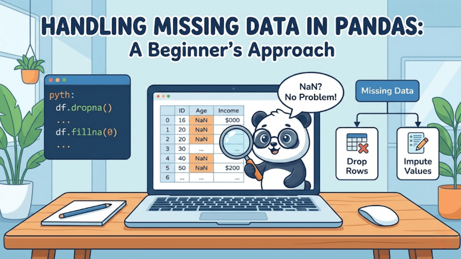
Missing data in Pandas is represented by NaN (Not a Number) for numeric columns and None or NaT for object and datetime columns. Pandas provides a powerful toolkit — including isna(), dropna(), fillna(), and interpolate() — to detect, remove, and impute missing values so your data is clean and ready for analysis or machine learning.
Introduction: Why Missing Data Is One of Your Biggest Challenges
If there is one certainty in data science, it is this: real-world data is almost never complete. Whether you are working with survey responses where participants skipped questions, sensor data where a device went offline, medical records where tests were not performed, or e-commerce logs where a session ended before checkout — missing values are everywhere.
Missing data is not merely an inconvenience. It can silently corrupt your analyses, cause machine learning models to crash during training, introduce subtle biases into your results, and lead to conclusions that do not reflect reality. A model trained on data where missing values were handled carelessly can underperform dramatically compared to one where the same data was cleaned thoughtfully.
Pandas, the most widely used data manipulation library in Python, provides a rich set of tools for detecting, understanding, and handling missing values. These tools are beginner-friendly on the surface but have enough depth to satisfy even advanced practitioners. This article will take you from zero — understanding what missing data is and how Pandas represents it — all the way to practical strategies for cleaning your datasets in real-world scenarios.
By the end of this guide, you will know how to detect where missing values live in your data, understand the three major strategies for handling them (dropping, filling, and interpolating), choose the right strategy for different types of data and contexts, and apply these skills confidently in your own projects.
1. How Pandas Represents Missing Data
Before you can handle missing data, you need to understand how Pandas thinks about it internally. Pandas uses several special values to represent “no data here”:
NaN (Not a Number): This is a special floating-point value defined by the IEEE 754 standard. It is the most common representation of missing data in Pandas for numeric columns. Technically, NaN is a float, which is why a column of integers that contains missing values often gets converted to float64 when loaded into Pandas.
None: Python’s built-in null object. Pandas accepts None as a missing value marker, especially in object-dtype columns (columns containing strings or mixed types). In numeric contexts, Pandas typically converts None to NaN.
NaT (Not a Time): Pandas uses NaT specifically for missing values in datetime columns. If you have a column of dates and some entries are missing, they will appear as NaT.
pd.NA: Introduced in newer versions of Pandas as a consistent missing value indicator that works across all nullable integer, boolean, and string dtypes. You will encounter it when working with Int64, boolean, or StringDtype columns.
Here is a quick demonstration of how these appear in practice:
import pandas as pd
import numpy as np

df = pd.DataFrame({
    'numeric':   [1.0, np.nan, 3.0, np.nan, 5.0],
    'text':      ['apple', None, 'cherry', 'date', None],
    'dates':     pd.to_datetime(['2024-01-01', None, '2024-01-03', None, '2024-01-05']),
    'integers':  pd.array([1, pd.NA, 3, pd.NA, 5], dtype='Int64')
})

print(df)
print('\nData types:')
print(df.dtypes)Output:
   numeric    text      dates  integers
0      1.0   apple 2024-01-01         1
1      NaN    None        NaT      <NA>
2      3.0  cherry 2024-01-03         3
3      NaN    date        NaT      <NA>
4      5.0    None 2024-01-05         5

Data types:
numeric             float64
text                 object
dates        datetime64[ns]
integers Int64Notice that None in the text column displays as None, NaN appears in the numeric column, NaT appears in the dates column, and <NA> appears in the nullable integer column. All of these represent missing data, just in different contexts.
2. Detecting Missing Data
The first step in handling missing data is knowing where it exists. Pandas provides several methods for this purpose, each giving you a different level of detail.
2.1 The isna() and isnull() Methods
The isna() method (and its alias isnull()) returns a DataFrame or Series of the same shape filled with True where values are missing and False where they are not. These two methods are identical — isnull() exists for compatibility with older code.
import pandas as pd
import numpy as np

df = pd.DataFrame({
    'name':   ['Alice', 'Bob', None, 'Diana', 'Edward'],
    'age':    [28, np.nan, 25, np.nan, 40],
    'salary': [85000, 72000, np.nan, 65000, 95000]
})

print(df.isna())
#     name    age  salary
# 0  False  False   False
# 1  False   True   False
# 2   True  False    True
# 3  False   True   False
# 4 False False FalseThis boolean DataFrame is useful for further filtering, but for a quick summary, you will more often want to know the count of missing values per column.
2.2 Counting Missing Values Per Column
Chaining .isna() with .sum() gives you the total count of missing values in each column, since True counts as 1 and False as 0:
print(df.isna().sum())
# name      1
# age       2
# salary    1
# dtype: int64To see the percentage of missing values (often more meaningful in large datasets), divide by the total number of rows:
missing_pct = (df.isna().sum() / len(df)) * 100
print(missing_pct.round(2))
# name      20.0
# age       40.0
# salary    20.0
# dtype: float64This tells you that 40% of age values and 20% of name and salary values are missing — immediately actionable information.
2.3 Building a Complete Missing Data Summary
For a professional-quality overview of your dataset’s missing values, you can build a summary DataFrame:
def missing_data_summary(df):
    """Generate a comprehensive missing data report."""
    total = df.shape[0]
    missing_count = df.isna().sum()
    missing_pct   = (missing_count / total * 100).round(2)
    dtype_info    = df.dtypes

    summary = pd.DataFrame({
        'Missing Count':   missing_count,
        'Missing %':       missing_pct,
        'Dtype':           dtype_info
    })

    # Only show columns that actually have missing values
    summary = summary[summary['Missing Count'] > 0]
    summary = summary.sort_values('Missing %', ascending=False)
    return summary

# Apply to a larger sample dataset
data = {
    'CustomerID':  range(1, 11),
    'Age':         [25, np.nan, 35, 28, np.nan, 42, np.nan, 33, 27, np.nan],
    'Income':      [50000, 62000, np.nan, 45000, 71000, np.nan, 58000, np.nan, 49000, 83000],
    'Gender':      ['M', 'F', None, 'M', 'F', 'M', None, 'F', 'M', None],
    'PurchaseAmt': [120.5, 89.0, 234.0, np.nan, 67.5, 310.0, np.nan, 150.0, 95.5, 420.0]
}

customers = pd.DataFrame(data)
print(missing_data_summary(customers))

#              Missing Count  Missing %   Dtype
# Age                      4       40.0   float64
# Gender                   3       30.0    object
# Income                   3       30.0   float64
# PurchaseAmt 2 20.0 float64This summary is an excellent starting point for any data cleaning workflow. By sorting by missing percentage, you immediately know which columns need the most attention.
2.4 Visualizing Missing Data Patterns
For larger datasets, a visual representation of missing values helps you spot patterns — for instance, whether certain columns tend to be missing together (which could indicate a systemic data collection issue):
import pandas as pd
import numpy as np

# Heatmap of missing values using a simple text representation
df_large = pd.DataFrame(
    np.random.choice([1.0, np.nan], size=(10, 5), p=[0.7, 0.3]),
    columns=['Col_A', 'Col_B', 'Col_C', 'Col_D', 'Col_E']
)

# Show which cells are missing (True = missing)
print(df_large.isna().astype(int))
#    Col_A  Col_B  Col_C  Col_D  Col_E
# 0      0      1      0      0      1
# 1      1      0      0      1      0
# ...In a full data science environment with Matplotlib or Seaborn, you would create a heatmap: sns.heatmap(df.isna(), cbar=False, cmap='viridis'). The resulting visual makes it immediately clear whether missing values are scattered randomly or clustered in particular rows or columns.
3. Understanding Types of Missingness
Before deciding how to handle missing data, it helps enormously to understand why data is missing. Statisticians classify missing data into three categories, and the appropriate handling strategy depends heavily on which category applies to your data.
3.1 Missing Completely at Random (MCAR)
Data is MCAR when the probability of a value being missing has nothing to do with the value itself or any other variable. An example: a sensor randomly malfunctions and fails to record a reading, with no relationship to what the reading would have been. With MCAR data, any complete-case analysis (simply dropping missing rows) produces unbiased results, though you lose statistical power proportional to the amount of data dropped.
3.2 Missing at Random (MAR)
Data is MAR when the probability of a value being missing depends on other observed variables, but not on the missing value itself. Example: older survey respondents are less likely to report their income, but among respondents of the same age, whether income is missing has nothing to do with the actual income amount. MAR is the most common situation in practice and supports sophisticated imputation methods.
3.3 Missing Not at Random (MNAR)
Data is MNAR when the probability of a value being missing depends on the value that is missing. Example: very high-income individuals are more likely to decline reporting their income precisely because it is high. MNAR is the most challenging case — ignoring it can introduce serious bias into your analysis. It often requires domain expertise and specialized handling strategies.
Practical tip: In most beginner and intermediate data science projects, you can proceed with reasonable assumptions about the nature of missingness. However, for any analysis where the results will influence important decisions — medical, financial, or policy-related — understanding the type of missingness is critical.
4. Strategy 1: Dropping Missing Values with dropna()
The simplest strategy for handling missing data is to remove rows or columns that contain missing values. Pandas makes this easy with the dropna() method. However, dropping data should be done thoughtfully — you can easily discard too much information if you are not careful.
4.1 Dropping Rows with Any Missing Value
import pandas as pd
import numpy as np

df = pd.DataFrame({
    'name':   ['Alice', 'Bob', None, 'Diana', 'Edward'],
    'age':    [28, np.nan, 25, np.nan, 40],
    'salary': [85000, 72000, np.nan, 65000, 95000]
})

# Drop any row that has at least one missing value
df_clean = df.dropna()
print(df_clean)
#     name   age   salary
# 0  Alice  28.0  85000.0
# 4 Edward 40.0 95000.0With how='any' (the default), dropna() removes any row that contains even a single NaN. In our small example, this leaves only 2 out of 5 rows — a significant loss. In large datasets with many columns, dropping rows with any missing value can eliminate the vast majority of your data.
4.2 Dropping Rows Only When ALL Values Are Missing
# Drop only rows where EVERY value is missing
df_less_aggressive = df.dropna(how='all')
print(df_less_aggressive)
# All rows are retained in this example since no row is entirely NaNThe how='all' option is much less aggressive — it only removes rows (or columns) where every single value is missing. This is useful for cleaning up completely empty rows that sometimes appear in data exports.
4.3 Dropping Columns Instead of Rows
You can also drop columns (rather than rows) that contain missing values by using axis=1:
# Drop any column that has at least one missing value
df_no_missing_cols = df.dropna(axis=1)
print(df_no_missing_cols)
# Empty DataFrame (all columns have at least one missing value in this example)4.4 The thresh Parameter: Setting a Minimum Threshold
The thresh parameter is one of the most useful options in dropna(). It lets you specify the minimum number of non-missing values a row (or column) must have to be kept:
df = pd.DataFrame({
    'A': [1,    np.nan, 3,    np.nan, np.nan],
    'B': [4,    5,      np.nan, np.nan, np.nan],
    'C': [7,    8,      9,    np.nan, np.nan],
    'D': [10,   11,     12,   13,     np.nan]
})

# Keep only rows with at least 3 non-missing values
df_thresh = df.dropna(thresh=3)
print(df_thresh)
#      A     B     C     D
# 0  1.0   4.0   7.0  10.0
# 1  NaN   5.0   8.0  11.0
# 2 3.0 NaN 9.0 12.0This approach strikes a balance: rows with too many missing values are removed, but rows with only one or two missing values are kept for imputation.
4.5 The subset Parameter: Dropping Based on Specific Columns
Sometimes you only care about missing values in certain critical columns:
customers = pd.DataFrame({
    'customer_id': [1, 2, 3, 4, 5],
    'email':       ['a@x.com', None, 'c@x.com', None, 'e@x.com'],
    'age':         [25, 30, np.nan, 28, 35],
    'purchase':    [100, 200, 150, np.nan, 300]
})

# Only drop rows where 'email' is missing (it's the critical identifier)
df_email_required = customers.dropna(subset=['email'])
print(df_email_required)
#    customer_id     email   age  purchase
# 0            1  a@x.com  25.0     100.0
# 2            3  c@x.com   NaN     150.0
# 4 5 e@x.com 35.0 300.0Using subset lets you be surgical about which columns trigger row removal, preserving as much data as possible.
4.6 When Should You Drop Missing Data?
Dropping is appropriate when the percentage of missing values is small (generally under 5% of the dataset), when the data appears to be MCAR (missing completely at random), when the column with missing values is not critical to your analysis, or when you have a very large dataset where losing some rows is inconsequential.
Dropping is not appropriate when you have a significant percentage of missing values, when the missing pattern is not random (MAR or MNAR), or when the column contains critical information that cannot be reconstructed.
5. Strategy 2: Filling Missing Values with fillna()
Rather than removing missing data, you can replace it with a reasonable substitute value. This is called imputation, and Pandas provides the fillna() method as the primary tool for it.
5.1 Filling with a Constant Value
The simplest form of imputation replaces all missing values with a single constant:
import pandas as pd
import numpy as np

df = pd.DataFrame({
    'product': ['Laptop', 'Mouse', 'Monitor', 'Keyboard', 'Webcam'],
    'price':   [999.99, np.nan, 349.99, np.nan, 79.99],
    'in_stock': [True, np.nan, True, False, np.nan]
})

# Fill numeric missing with 0 (useful for quantities, counts)
df_filled = df.copy()
df_filled['price'] = df['price'].fillna(0)
print(df_filled)Filling with a constant is most appropriate for categorical or count data where 0 or “Unknown” is a meaningful substitute. For numeric measurements like prices or ages, filling with 0 is usually wrong because it distorts the distribution.
5.2 Filling with Summary Statistics
For numeric columns, filling with the mean or median of the existing values is a widely used approach:
df = pd.DataFrame({
    'age':    [25, np.nan, 35, 28, np.nan, 42, 33, np.nan, 27, 38],
    'salary': [50000, 62000, np.nan, 45000, 71000, np.nan, 58000, 49000, np.nan, 83000]
})

# Fill age with median (more robust to outliers than mean)
age_median = df['age'].median()
df['age_filled'] = df['age'].fillna(age_median)

# Fill salary with mean
salary_mean = df['salary'].mean()
df['salary_filled'] = df['salary'].fillna(salary_mean)

print(f'Age median used for imputation: {age_median}')
print(f'Salary mean used for imputation: {salary_mean:.2f}')
print(df[['age', 'age_filled', 'salary', 'salary_filled']])Mean vs Median — when to use which:
| Situation | Recommended Statistic |
|---|---|
| Data is approximately normally distributed | Mean |
| Data has significant outliers (e.g., income, house prices) | Median |
| Data is right-skewed (many small values, few large ones) | Median |
| Column represents a count without extreme values | Mean or Median |
| Column represents a proportion (0–1) | Mean |
| Categorical column (mode imputation) | Mode |
5.3 Filling Categorical Columns with Mode
For text or categorical columns, the most common value (mode) is typically the best simple imputation:
df = pd.DataFrame({
    'city':       ['New York', 'Chicago', None, 'New York', 'Chicago', None, 'New York'],
    'product':    ['Laptop', None, 'Monitor', 'Laptop', None, 'Mouse', 'Laptop'],
    'rating':     [5, 4, np.nan, 5, 3, np.nan, 4]
})

# Fill categorical columns with mode
city_mode = df['city'].mode()[0]     # mode() returns a Series; take first element
product_mode = df['product'].mode()[0]

df['city']    = df['city'].fillna(city_mode)
df['product'] = df['product'].fillna(product_mode)

print(f'City mode: {city_mode}')
print(f'Product mode: {product_mode}')
print(df)Note that mode() returns a Series (because there could be multiple modes), so you need to index it with [0] to get the single most common value.
5.4 Forward Fill and Backward Fill
Two powerful and often overlooked imputation strategies are forward fill (ffill) and backward fill (bfill). These methods propagate the last known value forward (or the next known value backward) to fill gaps.
These strategies are especially useful for time series data, where it is reasonable to assume that a missing value is similar to the most recently observed value:
import pandas as pd
import numpy as np

# Stock price time series with missing values
dates = pd.date_range('2024-01-01', periods=10, freq='B')
stock_prices = pd.Series(
    [150.0, np.nan, np.nan, 153.5, np.nan, 155.0, np.nan, 157.2, np.nan, 160.0],
    index=dates,
    name='Price'
)

print("Original:")
print(stock_prices)

print("\nForward Fill (carry last known value forward):")
print(stock_prices.ffill())

print("\nBackward Fill (use next known value to fill backward):")
print(stock_prices.bfill())

print("\nForward Fill then Backward Fill (handles edges):")
print(stock_prices.ffill().bfill())Output:
Original:
2024-01-01    150.0
2024-01-02      NaN
2024-01-03      NaN
2024-01-04    153.5
2024-01-05      NaN
...

Forward Fill:
2024-01-01    150.0
2024-01-02    150.0   ← carried from Jan 1
2024-01-03    150.0   ← carried from Jan 1
2024-01-04    153.5
2024-01-05    153.5   ← carried from Jan 4
...You can also limit how many consecutive NaN values get filled using the limit parameter:
# Fill at most 1 consecutive NaN (leave longer gaps unfilled)
print(stock_prices.ffill(limit=1))
# 2024-01-01    150.0
# 2024-01-02    150.0   ← filled (1 consecutive)
# 2024-01-03      NaN   ← not filled (would be 2nd consecutive)
# 2024-01-04 153.55.5 Group-Aware Imputation
One of the most powerful imputation techniques — and one that beginners often overlook — is filling missing values using the group mean or median rather than the overall mean. This produces much more accurate imputations when values differ significantly across groups:
df = pd.DataFrame({
    'department': ['Engineering', 'Engineering', 'Marketing', 'Marketing',
                   'Engineering', 'Marketing', 'Engineering', 'Marketing'],
    'salary':     [95000, np.nan, 65000, np.nan, 88000, 71000, np.nan, 68000]
})

# The overall mean salary would be a poor imputation for
# Engineering (high-paid) and Marketing (lower-paid) combined.

# Instead, fill with group-specific median
df['salary_imputed'] = df.groupby('department')['salary'].transform(
    lambda x: x.fillna(x.median())
)

print(df)
#    department   salary  salary_imputed
# 0  Engineering  95000.0         95000.0
# 1  Engineering      NaN         91500.0  ← Engineering median
# 2    Marketing  65000.0         65000.0
# 3    Marketing      NaN         66500.0  ← Marketing median
# 4  Engineering  88000.0         88000.0
# 5    Marketing  71000.0         71000.0
# 6  Engineering      NaN         91500.0  ← Engineering median
# 7 Marketing 68000.0 68000.0The .transform() method applies the lambda function within each group and returns a result with the same index as the original DataFrame, making it perfect for group-aware imputation.
6. Strategy 3: Interpolating Missing Values
For time series and ordered sequential data, interpolation is often more accurate than simple mean or median imputation. Rather than using a constant value, interpolation estimates the missing value by looking at neighboring values and fitting a mathematical function between them.
6.1 Linear Interpolation
Linear interpolation assumes that missing values lie on a straight line between the two neighboring known values:
import pandas as pd
import numpy as np

# Temperature readings with gaps
temps = pd.Series([20.0, np.nan, np.nan, 23.0, np.nan, 25.5, np.nan, 28.0])

print("Original:", temps.values)
print("Linear interpolation:", temps.interpolate(method='linear').values)

# Output:
# Original: [20.  nan  nan  23.  nan  25.5  nan  28. ]
# Linear: [20. 21. 22. 23. 24.25 25.5 26.75 28. ]With linear interpolation, the two missing values between 20.0 and 23.0 are estimated as 21.0 and 22.0 (equally spaced steps). This makes intuitive sense for smoothly varying data like temperatures, sensor readings, or financial metrics.
6.2 Polynomial and Spline Interpolation
For data that follows a non-linear curve, polynomial or spline interpolation can produce more accurate estimates:
import pandas as pd
import numpy as np

# A curve-like pattern
values = pd.Series([1.0, np.nan, 9.0, np.nan, 25.0, np.nan, 49.0])

print("Linear:", values.interpolate(method='linear').values)
print("Polynomial (order 2):", values.interpolate(method='polynomial', order=2).values)
print("Spline (order=3):", values.interpolate(method='spline', order=3).values)Higher-order methods fit the data more precisely when the underlying trend is non-linear, but they require the scipy library to be installed. For most beginner applications, linear interpolation is sufficient and safe.
6.3 Time-Aware Interpolation
When your data has a DatetimeIndex with irregular time gaps, time-aware interpolation accounts for the actual temporal distance between observations rather than treating all gaps as equal:
import pandas as pd
import numpy as np

# Irregular time stamps — note the unequal gaps
index = pd.to_datetime(['2024-01-01', '2024-01-02', '2024-01-05', '2024-01-06'])
values = pd.Series([10.0, np.nan, np.nan, 40.0], index=index)

print("Index-aware interpolation:")
print(values.interpolate(method='index'))
# Accounts for the fact that Jan 2 to Jan 5 is a 3-day gap
# 2024-01-01    10.000000
# 2024-01-02    20.000000   ← 1/4 of the way between Jan 1 and Jan 6
# 2024-01-05    36.666667   ← 4/5 of the way
# 2024-01-06 40.0000006.4 Limiting Interpolation
Just like fillna(), the interpolate() method supports a limit parameter to control how many consecutive values get filled:
values = pd.Series([1.0, np.nan, np.nan, np.nan, np.nan, 10.0])

# Only fill up to 2 consecutive NaN values from each known point
print(values.interpolate(limit=2))
# 0     1.0
# 1     2.8    ← filled
# 2     4.6    ← filled (limit reached)
# 3     NaN    ← not filled
# 4     NaN    ← not filled
# 5 10.0This is useful when you want to fill short gaps confidently but leave long gaps unfilled (or handle them separately), acknowledging that interpolation becomes less reliable over longer stretches.
7. Advanced: Using Scikit-Learn for Imputation
For machine learning pipelines, Pandas-based imputation has a significant limitation: the imputation statistics (mean, median, mode) are calculated on the training data. If you apply them naively to test data, you risk data leakage — allowing information from the test set to influence the training process. Scikit-learn’s imputation tools solve this problem cleanly.
7.1 SimpleImputer
SimpleImputer from sklearn.impute is the direct machine-learning-pipeline equivalent of Pandas fillna():
import pandas as pd
import numpy as np
from sklearn.impute import SimpleImputer
from sklearn.model_selection import train_test_split

# Create a dataset with missing values
df = pd.DataFrame({
    'age':    [25, np.nan, 35, 28, np.nan, 42, 33, np.nan, 27, 38],
    'income': [50000, 62000, np.nan, 45000, 71000, np.nan, 58000, 49000, np.nan, 83000],
    'score':  [7.5, 8.2, np.nan, 6.9, 8.8, 7.1, np.nan, 7.6, 6.5, 9.1]
})

X = df[['age', 'income', 'score']]

# Split BEFORE imputation to avoid data leakage
X_train, X_test = train_test_split(X, test_size=0.3, random_state=42)

# Create and fit imputer on training data ONLY
imputer = SimpleImputer(strategy='median')
imputer.fit(X_train)

# Transform both train and test sets
X_train_imputed = imputer.transform(X_train)
X_test_imputed  = imputer.transform(X_test)

print("Training medians used for imputation:")
print(dict(zip(X.columns, imputer.statistics_)))7.2 KNNImputer
The K-Nearest Neighbors imputer is a more sophisticated approach that uses the values of similar rows (neighbors) to estimate missing values:
from sklearn.impute import KNNImputer

# KNN imputation: use 3 nearest neighbors
knn_imputer = KNNImputer(n_neighbors=3)
X_knn_imputed = knn_imputer.fit_transform(X)

print("KNN Imputed values:")
print(pd.DataFrame(X_knn_imputed, columns=X.columns).round(2))KNN imputation is more computationally expensive than simple mean/median imputation, but it often produces more accurate results because it considers the relationships between features rather than filling each column independently.
8. Practical Workflow: A Complete Missing Data Cleaning Pipeline
Let us put everything together in a realistic end-to-end workflow for a customer dataset:
import pandas as pd
import numpy as np

# ── 1. Load / simulate dataset ──────────────────────────────────────────────
np.random.seed(42)
n = 200

data = {
    'customer_id': range(1, n + 1),
    'age':         np.where(
                       np.random.rand(n) < 0.12,
                       np.nan,
                       np.random.randint(18, 70, n).astype(float)
                   ),
    'gender':      np.where(
                       np.random.rand(n) < 0.08,
                       None,
                       np.random.choice(['M', 'F', 'Other'], n)
                   ),
    'income':      np.where(
                       np.random.rand(n) < 0.15,
                       np.nan,
                       np.random.normal(60000, 20000, n).round(2)
                   ),
    'purchase_amt':np.where(
                       np.random.rand(n) < 0.05,
                       np.nan,
                       np.random.exponential(150, n).round(2)
                   ),
    'region':      np.where(
                       np.random.rand(n) < 0.10,
                       None,
                       np.random.choice(['North', 'South', 'East', 'West'], n)
                   ),
}

df = pd.DataFrame(data)

# ── 2. Audit missing data ────────────────────────────────────────────────────
print("=== STEP 1: Missing Data Audit ===")
missing_summary = pd.DataFrame({
    'Missing Count': df.isna().sum(),
    'Missing %':     (df.isna().sum() / len(df) * 100).round(2)
})
print(missing_summary[missing_summary['Missing Count'] > 0])

# ── 3. Drop rows missing critical identifier (customer_id always present) ───
print("\n=== STEP 2: No critical-column drops needed (customer_id complete) ===")

# ── 4. Impute numeric columns ────────────────────────────────────────────────
print("\n=== STEP 3: Numeric Imputation ===")

# Age: use median (more robust to skew)
age_median = df['age'].median()
df['age'] = df['age'].fillna(age_median)
print(f"Age imputed with median: {age_median:.1f}")

# Income: group-aware imputation — use region median where available
# First, for rows where region is also missing, use overall median
overall_income_median = df['income'].median()
df['income'] = df.groupby('region')['income'].transform(
    lambda x: x.fillna(x.median())
)
# Handle any remaining NaN (rows where region was also missing)
df['income'] = df['income'].fillna(overall_income_median)
print(f"Income imputed with region-grouped medians (fallback: {overall_income_median:.2f})")

# Purchase amount: low missing rate (5%), fill with median
purchase_median = df['purchase_amt'].median()
df['purchase_amt'] = df['purchase_amt'].fillna(purchase_median)
print(f"Purchase amount imputed with median: {purchase_median:.2f}")

# ── 5. Impute categorical columns ────────────────────────────────────────────
print("\n=== STEP 4: Categorical Imputation ===")

gender_mode = df['gender'].mode()[0]
region_mode = df['region'].mode()[0]

df['gender'] = df['gender'].fillna(gender_mode)
df['region'] = df['region'].fillna(region_mode)

print(f"Gender imputed with mode: {gender_mode}")
print(f"Region imputed with mode: {region_mode}")

# ── 6. Verify no missing values remain ──────────────────────────────────────
print("\n=== STEP 5: Verification ===")
remaining_missing = df.isna().sum().sum()
print(f"Total remaining missing values: {remaining_missing}")
print(df.info())This pipeline demonstrates a professional approach: audit first, choose the appropriate strategy for each column based on its type and missingness pattern, apply imputation, and verify the result.
9. Common Mistakes and How to Avoid Them
9.1 Imputing Before Splitting Train and Test Sets
This is the most dangerous mistake in machine learning workflows. If you compute the mean or median on the full dataset (including test data) before splitting, information from the test set leaks into your model — making your cross-validation scores artificially optimistic. Always split your data first, then impute using statistics computed only from the training set.
9.2 Dropping Too Aggressively
Using df.dropna() without any arguments is tempting for its simplicity, but it can eliminate the majority of your dataset if any column has missing values. Always inspect df.isna().sum() first to understand the scope of missingness before deciding to drop.
9.3 Filling All Columns with the Same Value
Using df.fillna(0) on an entire DataFrame is rarely a good idea. A salary of 0, an age of 0, or a product rating of 0 are rarely meaningful substitutes — they distort distributions and mislead machine learning models. Choose your imputation strategy column by column, based on the semantics of each variable.
9.4 Forgetting to Check for NaN in Boolean Operations
NaN in Pandas is not equal to anything, including itself. This means np.nan == np.nan returns False, and filtering with df[df['col'] == np.nan] will never find any rows. Always use isna() or notna() for missing value checks:
# WRONG — never finds any NaN rows
wrong = df[df['age'] == np.nan]    # Empty DataFrame

# CORRECT
correct_missing = df[df['age'].isna()]
correct_present = df[df['age'].notna()]9.5 Ignoring the notna() Method
The complement of isna() is notna() (or notnull()). It is just as useful and often more readable than ~df.isna():
# These are equivalent, but notna() is more readable
df[df['salary'].notna()]
df[~df['salary'].isna()]10. Choosing the Right Strategy: A Decision Guide
Deciding how to handle missing data is as much art as science, informed by the nature of your data and the goals of your analysis. Here is a practical decision framework:
Use dropna() when:
- Missing values are less than 5% of your data
- You have strong reason to believe the data is MCAR
- The column with missing values is not critical to your analysis
- You have a very large dataset where data loss is inconsequential
Use mean/median fillna() when:
- Missing rate is moderate (5–30%)
- The column is numeric
- You need a quick, reasonable baseline imputation
- Use median for skewed distributions (income, prices, house sizes), mean for roughly symmetric distributions
Use mode fillna() when:
- The column is categorical or ordinal
- The most common category is a reasonable default
Use forward/backward fill (ffill/bfill) when:
- Your data is a time series or has a natural ordering
- Missing values likely reflect a continuation of the previous state
- Gaps are short relative to the overall series length
Use interpolate() when:
- Your data has a smooth underlying trend
- The data is ordered (time series, spatial data)
- Neighboring values are more informative than the global mean
Use group-aware imputation when:
- Your data has natural groupings (department, region, product category)
- Values differ significantly across groups
- You want imputed values to respect the within-group distribution
Use KNN or model-based imputation when:
- Your data has complex relationships between features
- You want the most accurate possible imputation and have compute budget
- You are building a high-stakes production machine learning model
Conclusion: Clean Data Is the Foundation of Good Data Science
Handling missing data well is one of the most important and underappreciated skills in a data scientist’s toolkit. Unlike the more glamorous aspects of machine learning — model selection, hyperparameter tuning, deep learning architectures — data cleaning rarely gets attention in tutorials or course curricula. Yet in practice, the quality of your data cleaning often determines the quality of your results more than any other single factor.
In this article, you learned how Pandas represents missing data through NaN, None, NaT, and pd.NA. You learned how to detect missing values at the individual cell level with isna(), at the column level with isna().sum(), and visually through heatmaps. You explored three major handling strategies — dropping with dropna(), filling with fillna(), and interpolating with interpolate() — and saw concrete examples of when each is appropriate. You also glimpsed more advanced techniques including group-aware imputation and scikit-learn’s SimpleImputer and KNNImputer for production pipelines.
Most importantly, you now understand that handling missing data is not about applying one universal recipe. It requires judgment, an understanding of why data is missing in the first place, and thoughtful consideration of how each choice will affect your downstream analysis.
In the next article, you will build on these skills by learning about grouping and aggregating data with Pandas — techniques that unlock powerful summaries and insights from your cleaned datasets.
Key Takeaways
- Pandas represents missing data as
NaN(numeric),None(object),NaT(datetime), andpd.NA(nullable types). - Use
df.isna().sum()and(df.isna().sum() / len(df) * 100)to audit the count and percentage of missing values per column. dropna()removes rows or columns with missing values; control it withhow,thresh, andsubsetparameters.fillna()replaces missing values with a constant, mean, median, mode, or propagated value; choose the method based on the column’s data type and distribution.- Forward fill (
ffill) and backward fill (bfill) are ideal for time series data where values carry over between observations. interpolate()estimates missing values using surrounding data points; usemethod='linear'for smooth trends andmethod='index'for irregular time series.- Group-aware imputation using
groupby().transform()produces more accurate imputations when values differ across categories. - Always split data into train and test sets before computing imputation statistics to avoid data leakage.
- Never use
df['col'] == np.nanto detect missing values — always usedf['col'].isna()instead. - Match your imputation strategy to your data: use median for skewed numeric data, mode for categorical data, and interpolation for ordered sequential data.