Logistic regression is a supervised machine learning algorithm used for classification that predicts the probability of an example belonging to a class. Despite its name containing “regression,” it is a classification algorithm — it applies the sigmoid function to a linear combination of features to squash outputs into the range (0, 1), producing a probability. For binary classification, examples with predicted probability above 0.5 are assigned to class 1, and below 0.5 to class 0. Logistic regression is the foundation of classification in machine learning and a direct conceptual bridge to neural network output layers.
Introduction: From Predicting Numbers to Predicting Categories
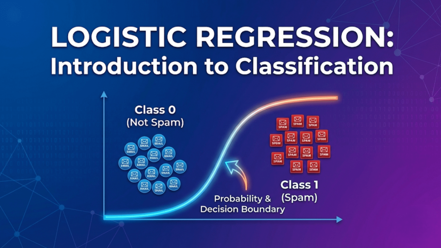
Linear regression predicts continuous numbers: house prices, temperatures, salaries. But many real-world problems require predicting categories: will this email be spam or not? Will this tumor be malignant or benign? Will this customer churn or stay? Will this loan default or be repaid?
These are classification problems — the output is a discrete category, not a continuous number. Plugging them into linear regression creates an immediate problem: linear regression predicts any real number, from negative infinity to positive infinity, but class labels are discrete values like 0 and 1. Predicting 2.7 or −0.3 for a binary outcome is meaningless.
Logistic regression solves this elegantly. It takes the same linear combination of features used in linear regression — w₁x₁ + w₂x₂ + … + b — and passes it through a sigmoid function that squashes any real number into the range (0, 1). The output becomes a probability: “there is a 73% chance this email is spam.” Apply a decision threshold (typically 0.5), and you have a classification: spam or not spam.
This one modification — wrapping the linear function in a sigmoid — transforms regression into classification. It may seem like a small change, but it has profound implications for the cost function, the learning algorithm, and the interpretation of results.
Logistic regression is one of the most important algorithms in machine learning. It’s used across medicine (disease diagnosis), finance (credit scoring), marketing (customer churn), and countless other domains. More fundamentally, understanding logistic regression is essential for understanding neural networks: every binary classification neural network ends with a sigmoid-activated output neuron computing exactly what logistic regression computes.
This comprehensive guide covers logistic regression completely. You’ll learn why linear regression fails for classification, how the sigmoid function creates probabilities, the decision boundary, the log-loss cost function, gradient descent for logistic regression, multi-class extension, and complete Python implementations with worked examples.
Why Linear Regression Fails for Classification
Before building logistic regression, let’s understand exactly why linear regression is unsuitable.
Problem 1: Outputs Beyond [0, 1]
Binary classification: y ∈ {0, 1}

Linear regression: ŷ = wx + b can predict any value

Examples:
  ŷ = 1.7  → Probability > 1? Impossible.
  ŷ = −0.4 → Negative probability? Impossible.
  ŷ = 0.3  → 30% chance — this one makes sense.

Only predictions in [0, 1] are valid probabilities.
Linear regression doesn't guarantee this.Problem 2: Inappropriate Cost Function
If we use MSE with binary labels (0 or 1):
  Outliers (points far from boundary) dominate
  Cost function is non-convex for classification
  Gradient descent may find poor solutions
Training becomes unreliableProblem 3: Sensitive to Outliers
Dataset: All tumors are benign (y=0) for small masses,
         malignant (y=1) for large masses.

Linear fit works reasonably until...
One extreme outlier (very large benign tumor) is added.
Linear regression tilts to accommodate it,
misclassifying many non-outlier points.

Logistic regression is more robust in this scenario.Visualizing the Problem
y (class label)
1 │              ● ● ●
  │         ● ●
  │    ● ●
0 │● ●
  └────────────────────── x (feature)

Linear regression fit:
  Predicted line crosses y=0.5 somewhere
  But also predicts y=1.3 for large x (impossible probability)
  And y=-0.2 for small x (impossible probability)
  Sensitive to extreme points

Logistic regression:
  S-curve smoothly transitions from near-0 to near-1
  Always stays in valid probability range (0, 1)
Decision boundary where curve crosses 0.5The Sigmoid Function: The Heart of Logistic Regression
The sigmoid function transforms linear outputs into valid probabilities.
Definition
σ(z) = 1 / (1 + e^(−z))

Where:
z = linear combination: w₁x₁ + w₂x₂ + ... + b
e = Euler's number (≈ 2.718)
σ(z) = output probabilityKey Properties
Range: σ(z) ∈ (0, 1) — always a valid probability
σ(−∞) → 0   (as z → −∞, e^(−z) → ∞, so 1/(1+∞) → 0)
σ(0)   = 0.5 (at z=0, e^0=1, so 1/(1+1) = 0.5)
σ(+∞) → 1 (as z → +∞, e^(−z) → 0, so 1/(1+0) → 1)Shape: S-curve (sigmoid = S-shaped)
σ(z)
1.0 │                    ╭─────────────
    │                 ╭──╯
0.5 │──────────────╮─╯
    │           ╭──╯
0.0 │──────────╯
    └────────────────────────────── z
    −6  −4  −2   0   2   4   6
         ↑
σ(0) = 0.5 (decision boundary)Derivative (used in gradient descent):
σ'(z) = σ(z) × (1 − σ(z))

Beautiful property: derivative expressed in terms of the function itself.
At z=0: σ'(0) = 0.5 × 0.5 = 0.25 (maximum slope)Symmetry:
1 − σ(z) = σ(−z)

"Probability of class 0" = σ(−z)
"Probability of class 1" = σ(z)Numerical Examples
import numpy as np

def sigmoid(z):
    return 1 / (1 + np.exp(-z))

test_values = [-6, -3, -1, 0, 1, 3, 6]
for z in test_values:
print(f" σ({z:3d}) = {sigmoid(z):.4f}")Output:
  σ( -6) = 0.0025    ← Very likely class 0
  σ( -3) = 0.0474    ← Probably class 0
  σ( -1) = 0.2689    ← More likely class 0
  σ(  0) = 0.5000    ← Decision boundary
  σ(  1) = 0.7311    ← More likely class 1
  σ(  3) = 0.9526    ← Probably class 1
σ( 6) = 0.9975 ← Very likely class 1The Logistic Regression Model
The Equation
Step 1: Linear combination
z = w₁x₁ + w₂x₂ + ... + wₙxₙ + b
  = wᵀx + b

Step 2: Sigmoid activation
ŷ = σ(z) = 1 / (1 + e^(−z))

Output: ŷ = P(y=1 | x) — probability that example belongs to class 1Making a Classification Decision
Threshold τ (default = 0.5):
  If ŷ ≥ τ → Predict class 1
  If ŷ < τ → Predict class 0

Example:
  ŷ = 0.73 → 73% probability → Predict class 1
  ŷ = 0.31 → 31% probability → Predict class 0
ŷ = 0.50 → 50% probability → Predict class 1 (≥ threshold)Adjusting the threshold:
τ = 0.5: Default — balanced precision/recall
τ = 0.3: More sensitive — fewer false negatives (good for cancer detection)
τ = 0.7: More specific — fewer false positives (good for spam filter)

The threshold is chosen AFTER training based on application needs.The Decision Boundary
The decision boundary is where ŷ = 0.5, i.e., where z = 0:
z = wᵀx + b = 0
→ w₁x₁ + w₂x₂ + ... + wₙxₙ + b = 0

This is a hyperplane in feature space:
  1 feature: line     (x = −b/w₁)
  2 features: line    (w₁x₁ + w₂x₂ + b = 0)
n features: hyperplaneGeometric interpretation:
Feature 2
    │  ●●●
    │ ●●●●●          ← Class 1 (above boundary)
    │   ●●●
    │────────────     ← Decision boundary (z=0)
    │   ○○○
    │ ○○○○○○          ← Class 0 (below boundary)
    │   ○○○
    └────────────── Feature 1

The boundary line: w₁x₁ + w₂x₂ + b = 0The Cost Function: Binary Cross-Entropy (Log Loss)
MSE is wrong for logistic regression. The correct cost function is binary cross-entropy.
Why Not MSE?
If we used MSE with sigmoid:
  J(w,b) = (1/2m) Σ (σ(wᵀxᵢ + b) − yᵢ)²

Problem: Non-convex! Many local minima.
Gradient descent may get stuck, not converge to global minimum.

Need a convex cost function for reliable training.Binary Cross-Entropy (Log Loss)
Per-example loss:
L(ŷ, y) = −[y × log(ŷ) + (1−y) × log(1−ŷ)]

Where:
  ŷ = σ(z) = predicted probability
  y = true label (0 or 1)
log = natural logarithmUnderstanding the formula:
When y = 1 (true class is 1):
L = −log(ŷ)

If ŷ = 0.99 → L = −log(0.99) = 0.010  (low loss — correct and confident)
If ŷ = 0.50 → L = −log(0.50) = 0.693  (medium loss — correct but uncertain)
If ŷ = 0.01 → L = −log(0.01) = 4.605 (high loss — wrong and confident!)When y = 0 (true class is 0):
L = −log(1 − ŷ)

If ŷ = 0.01 → L = −log(0.99) = 0.010  (low loss — correct and confident)
If ŷ = 0.50 → L = −log(0.50) = 0.693  (medium loss)
If ŷ = 0.99 → L = −log(0.01) = 4.605 (high loss — wrong and confident!)Key behavior:
Confident and correct:  Very low loss (→ 0)
Uncertain (ŷ ≈ 0.5):    Moderate loss
Confident and wrong:    Very high loss (→ ∞)

Heavily penalizes confident wrong predictions.
This is exactly what we want!Total Cost Function
J(w, b) = −(1/m) × Σᵢ [yᵢ log(ŷᵢ) + (1−yᵢ) log(1−ŷᵢ)]

This is convex → single global minimum → gradient descent converges reliably.Numerical Example
def binary_cross_entropy(y_true, y_pred):
    """Compute binary cross-entropy loss."""
    eps = 1e-15  # Prevent log(0)
    y_pred = np.clip(y_pred, eps, 1 - eps)
    return -np.mean(y_true * np.log(y_pred) +
                    (1 - y_true) * np.log(1 - y_pred))

# Example: 5 predictions
y_true = np.array([1, 1, 0, 0, 1])
y_pred_good = np.array([0.9, 0.8, 0.1, 0.2, 0.7])   # Mostly correct
y_pred_bad  = np.array([0.3, 0.4, 0.7, 0.8, 0.2])   # Mostly wrong

print(f"Good predictions — Log Loss: {binary_cross_entropy(y_true, y_pred_good):.4f}")
print(f"Bad predictions — Log Loss: {binary_cross_entropy(y_true, y_pred_bad):.4f}")Output:
Good predictions — Log Loss: 0.2031
Bad  predictions — Log Loss: 1.6346

Lower is better. Good model has 8x lower loss.Gradient Descent for Logistic Regression
The Gradients
Partial derivatives of the cost function:
∂J/∂w = (1/m) × Xᵀ × (ŷ − y)
∂J/∂b = (1/m) × Σᵢ (ŷᵢ − yᵢ)

Where ŷᵢ = σ(wᵀxᵢ + b)Notice: Mathematically identical to linear regression gradients!
Linear regression:   ∂J/∂w = (1/m) Xᵀ(ŷ−y)   [ŷ = Xw+b]
Logistic regression: ∂J/∂w = (1/m) Xᵀ(ŷ−y)   [ŷ = σ(Xw+b)]

Same gradient formula — only difference is what ŷ means.Update Rules
w ← w − α × (1/m) × Xᵀ(σ(Xw+b) − y)
b ← b − α × (1/m) × Σᵢ (σ(wᵀxᵢ+b) − yᵢ)Complete Example: Predicting Diabetes
Dataset and Problem Setup
import numpy as np
import matplotlib.pyplot as plt
from sklearn.datasets import load_breast_cancer
from sklearn.model_selection import train_test_split
from sklearn.preprocessing import StandardScaler
from sklearn.metrics import (accuracy_score, classification_report,
                              confusion_matrix, roc_auc_score)

# Use breast cancer dataset (binary classification)
data = load_breast_cancer()
X, y = data.data, data.target
feature_names = data.feature_names

print(f"Dataset:  {X.shape[0]} examples, {X.shape[1]} features")
print(f"Classes:  {data.target_names}")
print(f"Class 0 (malignant): {(y==0).sum()}")
print(f"Class 1 (benign): {(y==1).sum()}")Output:
Dataset:  569 examples, 30 features
Classes:  ['malignant' 'benign']
Class 0 (malignant): 212
Class 1 (benign): 357From-Scratch Implementation
class LogisticRegressionScratch:
    """
    Binary logistic regression using gradient descent.
    Trained with binary cross-entropy (log loss).
    """

    def __init__(self, learning_rate=0.01,
                 n_iterations=1000, verbose=False):
        self.lr       = learning_rate
        self.n_iter   = n_iterations
        self.verbose  = verbose
        self.w_       = None
        self.b_       = None
        self.history_ = []

    @staticmethod
    def _sigmoid(z):
        # Numerically stable sigmoid
        return np.where(
            z >= 0,
            1 / (1 + np.exp(-z)),
            np.exp(z) / (1 + np.exp(z))
        )

    def _cost(self, y, y_pred):
        eps = 1e-15
        y_pred = np.clip(y_pred, eps, 1 - eps)
        return -np.mean(y * np.log(y_pred) +
                        (1 - y) * np.log(1 - y_pred))

    def fit(self, X, y):
        X = np.array(X, dtype=float)
        y = np.array(y, dtype=float)
        m, n = X.shape

        # Initialise
        self.w_ = np.zeros(n)
        self.b_ = 0.0
        self.history_ = []

        for i in range(self.n_iter):
            # Forward pass
            z     = X @ self.w_ + self.b_
            y_hat = self._sigmoid(z)

            # Cost
            cost = self._cost(y, y_hat)
            self.history_.append(cost)

            # Gradients
            error = y_hat - y
            dw = (1 / m) * (X.T @ error)
            db = (1 / m) * np.sum(error)

            # Update
            self.w_ -= self.lr * dw
            self.b_ -= self.lr * db

            if self.verbose and i % 200 == 0:
                print(f"  Iter {i:5d} | Loss: {cost:.4f}")

        return self

    def predict_proba(self, X):
        """Return probability of class 1."""
        X = np.array(X, dtype=float)
        z = X @ self.w_ + self.b_
        return self._sigmoid(z)

    def predict(self, X, threshold=0.5):
        """Return class labels (0 or 1)."""
        return (self.predict_proba(X) >= threshold).astype(int)

    def score(self, X, y):
        """Return accuracy."""
        return np.mean(self.predict(X) == y)

    def plot_loss(self):
        plt.figure(figsize=(8, 4))
        plt.plot(self.history_, color='steelblue', linewidth=1.5)
        plt.xlabel('Iteration')
        plt.ylabel('Binary Cross-Entropy Loss')
        plt.title('Training Loss Curve')
        plt.grid(True, alpha=0.3)
        plt.tight_layout()
plt.show()Train and Evaluate
# Split and scale
X_train, X_test, y_train, y_test = train_test_split(
    X, y, test_size=0.2, random_state=42, stratify=y
)

scaler = StandardScaler()
X_train_s = scaler.fit_transform(X_train)
X_test_s  = scaler.transform(X_test)

# Train from scratch
model_scratch = LogisticRegressionScratch(
    learning_rate=0.1, n_iterations=1000, verbose=True
)
model_scratch.fit(X_train_s, y_train)

# Evaluate
y_pred_train = model_scratch.predict(X_train_s)
y_pred_test  = model_scratch.predict(X_test_s)
y_prob_test  = model_scratch.predict_proba(X_test_s)

print(f"\nTraining accuracy: {accuracy_score(y_train, y_pred_train):.4f}")
print(f"Test accuracy:     {accuracy_score(y_test,  y_pred_test):.4f}")
print(f"Test ROC-AUC:      {roc_auc_score(y_test, y_prob_test):.4f}")

print("\nClassification Report:")
print(classification_report(y_test, y_pred_test,
                             target_names=data.target_names))

# Plot training curve
model_scratch.plot_loss()Expected Output:
  Iter     0 | Loss: 0.6931
  Iter   200 | Loss: 0.1823
  Iter   400 | Loss: 0.1345
  Iter   600 | Loss: 0.1201
  Iter   800 | Loss: 0.1156

Training accuracy: 0.9912
Test accuracy:     0.9737
Test ROC-AUC:      0.9968

Classification Report:
              precision    recall  f1-score   support
   malignant       0.96      0.98      0.97        43
      benign       0.99      0.97      0.98        71
accuracy 0.97 114Using Scikit-learn
from sklearn.linear_model import LogisticRegression

# scikit-learn includes regularization by default (C=1.0)
model_sklearn = LogisticRegression(
    C=1.0,           # Inverse regularization strength (larger = less regular)
    max_iter=1000,
    random_state=42
)
model_sklearn.fit(X_train_s, y_train)

y_pred_sk    = model_sklearn.predict(X_test_s)
y_prob_sk    = model_sklearn.predict_proba(X_test_s)[:, 1]

print(f"scikit-learn accuracy: {accuracy_score(y_test, y_pred_sk):.4f}")
print(f"scikit-learn ROC-AUC:  {roc_auc_score(y_test, y_prob_sk):.4f}")

# Feature importance (top 10 by absolute coefficient)
coef_df = pd.DataFrame({
    'feature':     feature_names,
    'coefficient': model_sklearn.coef_[0]
}).reindex(
    model_sklearn.coef_[0].argsort()[::-1]
)

import pandas as pd
coef_df = pd.DataFrame({
    'feature': feature_names,
    'coef': model_sklearn.coef_[0],
    'abs_coef': np.abs(model_sklearn.coef_[0])
}).sort_values('abs_coef', ascending=False)

print("\nTop 10 Most Important Features:")
print(coef_df[['feature', 'coef']].head(10).to_string(index=False))Visualizing the Decision Boundary (2D Example)
from sklearn.datasets import make_classification

# 2D dataset for visualization
X_2d, y_2d = make_classification(
    n_samples=300, n_features=2, n_redundant=0,
    n_informative=2, n_clusters_per_class=1,
    random_state=42
)

# Train logistic regression
scaler_2d = StandardScaler()
X_2d_s    = scaler_2d.fit_transform(X_2d)

model_2d  = LogisticRegression(C=1.0)
model_2d.fit(X_2d_s, y_2d)

# Create mesh grid for decision boundary
x_min, x_max = X_2d_s[:, 0].min() - 0.5, X_2d_s[:, 0].max() + 0.5
y_min, y_max = X_2d_s[:, 1].min() - 0.5, X_2d_s[:, 1].max() + 0.5
xx, yy = np.meshgrid(np.linspace(x_min, x_max, 200),
                     np.linspace(y_min, y_max, 200))
Z = model_2d.predict_proba(
    np.c_[xx.ravel(), yy.ravel()]
)[:, 1].reshape(xx.shape)

# Plot
fig, axes = plt.subplots(1, 2, figsize=(14, 5))

# Probability heatmap + boundary
ax = axes[0]
cf = ax.contourf(xx, yy, Z, levels=50, cmap='RdBu_r', alpha=0.8)
plt.colorbar(cf, ax=ax, label='P(class=1)')
ax.contour(xx, yy, Z, levels=[0.5], colors='black',
           linewidths=2, linestyles='--')
ax.scatter(X_2d_s[y_2d==0, 0], X_2d_s[y_2d==0, 1],
           c='blue', s=20, alpha=0.6, label='Class 0')
ax.scatter(X_2d_s[y_2d==1, 0], X_2d_s[y_2d==1, 1],
           c='red',  s=20, alpha=0.6, label='Class 1')
ax.set_title('Probability Map & Decision Boundary')
ax.set_xlabel('Feature 1')
ax.set_ylabel('Feature 2')
ax.legend()

# Hard predictions
ax = axes[1]
y_pred_2d = model_2d.predict(X_2d_s)
correct   = y_pred_2d == y_2d

ax.scatter(X_2d_s[correct, 0],  X_2d_s[correct, 1],
           c=y_2d[correct], cmap='RdBu', s=20, alpha=0.6, label='Correct')
ax.scatter(X_2d_s[~correct, 0], X_2d_s[~correct, 1],
           c='black', s=60, marker='x', linewidths=2, label='Misclassified')
ax.contour(xx, yy, Z, levels=[0.5], colors='black',
           linewidths=2, linestyles='--')
ax.set_title(f'Predictions  |  Accuracy: {accuracy_score(y_2d, y_pred_2d):.3f}')
ax.set_xlabel('Feature 1')
ax.set_ylabel('Feature 2')
ax.legend()

plt.tight_layout()
plt.show()Multi-Class Logistic Regression
Logistic regression extends to more than two classes.
One-vs-Rest (OvR)
Strategy: Train one binary classifier per class.
  Classifier 1: Class A vs. (B, C, D)
  Classifier 2: Class B vs. (A, C, D)
  Classifier 3: Class C vs. (A, B, D)
  Classifier 4: Class D vs. (A, B, C)

Prediction: Choose class with highest probability.Softmax Regression (Multinomial)
For K classes, use softmax instead of sigmoid:

P(y=k | x) = exp(wₖᵀx + bₖ) / Σⱼ exp(wⱼᵀx + bⱼ)

Properties:
  - All class probabilities sum to 1
  - Directly models multi-class probability
- More principled than OvRScikit-learn Multi-class Example
from sklearn.datasets import load_iris

iris = load_iris()
X_ir, y_ir = iris.data, iris.target

X_tr_ir, X_te_ir, y_tr_ir, y_te_ir = train_test_split(
    X_ir, y_ir, test_size=0.2, random_state=42
)
scaler_ir = StandardScaler()
X_tr_ir_s = scaler_ir.fit_transform(X_tr_ir)
X_te_ir_s = scaler_ir.transform(X_te_ir)

# Multinomial logistic regression
lr_multi = LogisticRegression(
    multi_class='multinomial',
    solver='lbfgs',
    max_iter=1000
)
lr_multi.fit(X_tr_ir_s, y_tr_ir)

print("Iris Dataset (3 classes):")
print(f"  Test accuracy: {lr_multi.score(X_te_ir_s, y_te_ir):.4f}")
print(f"  Coefficient shape: {lr_multi.coef_.shape}")
print("  (3 weight vectors — one per class)")

# Probability output
sample = X_te_ir_s[0:3]
probs  = lr_multi.predict_proba(sample)
print("\nProbabilities for first 3 test examples:")
print("  Setosa  Versicolor  Virginica  →  Prediction")
for p, pred in zip(probs, lr_multi.predict(sample)):
    print(f"  {p[0]:.3f}     {p[1]:.3f}       {p[2]:.3f}"
f" → {iris.target_names[pred]}")Regularization in Logistic Regression
Like linear regression, logistic regression benefits from regularization to prevent overfitting.
L2 Regularization (Ridge / Default in scikit-learn)
Cost with L2:
J(w,b) = −(1/m)Σ[y log(ŷ) + (1−y) log(1−ŷ)] + (λ/2m) Σ wᵢ²

Effect:
  Shrinks all weights toward zero
  Reduces model complexity
  Prevents overfitting

In scikit-learn: C = 1/λ
  Large C → weak regularization (complex model)
Small C → strong regularization (simple model)L1 Regularization (Lasso)
Cost with L1:
J(w,b) = −(1/m)Σ[y log(ŷ) + (1−y) log(1−ŷ)] + (λ/m) Σ |wᵢ|

Effect:
  Drives some weights to exactly zero
  Performs feature selection
Good for high-dimensional problemsChoosing Regularization Strength
from sklearn.model_selection import GridSearchCV

param_grid = {'C': [0.001, 0.01, 0.1, 1, 10, 100]}
grid = GridSearchCV(
    LogisticRegression(max_iter=1000),
    param_grid,
    cv=5,
    scoring='roc_auc'
)
grid.fit(X_train_s, y_train)

print(f"Best C:       {grid.best_params_['C']}")
print(f"Best ROC-AUC: {grid.best_score_:.4f}")Practical Diagnostics: Is the Model Working?
Calibration: Are Probabilities Meaningful?
from sklearn.calibration import calibration_curve

prob_true, prob_pred = calibration_curve(
    y_test, y_prob_sk, n_bins=10
)

plt.figure(figsize=(7, 5))
plt.plot(prob_pred, prob_true, 's-', color='steelblue',
         label='Logistic Regression')
plt.plot([0, 1], [0, 1], 'k--', label='Perfect calibration')
plt.xlabel('Mean Predicted Probability')
plt.ylabel('Fraction of Positives')
plt.title('Calibration Curve\n(Well-calibrated model follows diagonal)')
plt.legend()
plt.grid(True, alpha=0.3)
plt.tight_layout()
plt.show()Logistic regression is naturally well-calibrated — its predicted probabilities closely reflect true frequencies, unlike many other classifiers.
Logistic vs. Linear Regression: Key Differences
| Aspect | Linear Regression | Logistic Regression |
|---|---|---|
| Task | Regression (continuous output) | Classification (discrete output) |
| Output | Any real number (−∞, +∞) | Probability in (0, 1) |
| Activation | None (identity) | Sigmoid function |
| Decision rule | N/A | Threshold on probability |
| Cost function | MSE (Mean Squared Error) | Binary Cross-Entropy (Log Loss) |
| Cost landscape | Convex (bowl) | Convex (bowl) |
| Gradient formula | (1/m)Xᵀ(ŷ−y) | (1/m)Xᵀ(ŷ−y) — identical! |
| Interpretation | Predict numeric value | Predict class probability |
| Evaluation | R², RMSE, MAE | Accuracy, AUC, F1, Log Loss |
| Regularization | Ridge, Lasso | Ridge (C param), L1 |
| Link to NNs | Output layer (regression) | Output layer (binary classification) |
Conclusion: The Gateway to Classification
Logistic regression is simultaneously the simplest and one of the most important classification algorithms in machine learning. Simple because it adds just one transformation — the sigmoid function — to the linear model. Important because it introduces every concept that carries forward into more advanced classification: probability outputs, decision thresholds, log loss, the relationship between linear scores and class probabilities.
The deep connection to linear regression is striking and instructive:
Same linear combination: z = wᵀx + b appears in both models — logistic regression just applies sigmoid to it.
Same gradient formula: ∂J/∂w = (1/m)Xᵀ(ŷ−y) is mathematically identical for both, whether ŷ comes from identity or sigmoid.
Same optimization: Gradient descent with the same update rules trains both.
Same regularization: Ridge and Lasso apply identically; scikit-learn’s C parameter is simply 1/λ.
The only differences are the activation function (none vs. sigmoid), the cost function (MSE vs. log loss), and the interpretation (predicted value vs. predicted probability).
This connection extends forward to neural networks: a neural network performing binary classification is logistic regression with hidden layers. Its output neuron computes exactly σ(wᵀh + b) where h is the hidden layer’s output. The log loss used to train the network is the same binary cross-entropy. The gradient flows backward through the same sigmoid derivative.
Master logistic regression — understand its probability interpretation, its log loss cost function, its decision boundary, its regularization — and you understand the classification output layer of every neural network. That is the foundation this algorithm provides, and it makes it one of the most valuable algorithms to know deeply.