The cost function in linear regression is a mathematical formula that measures how wrong the model’s predictions are on the training data. The most common choice is Mean Squared Error (MSE): J(w,b) = (1/2m) × Σ(ŷᵢ − yᵢ)², which averages the squared differences between predicted and actual values. The cost function serves as the compass for learning — gradient descent iteratively adjusts model weights and bias in the direction that reduces cost, guiding the algorithm toward the parameter values that produce the best predictions.
Introduction: What Does “Learning” Really Mean?
When we say a machine learning model “learns from data,” what exactly is happening? It’s easy to imagine it as something mysterious — the model somehow absorbing knowledge from examples. But the reality is beautifully concrete: learning means minimizing a number.
That number is the cost function — a single scalar value that measures how wrong the model’s predictions currently are. At the start of training, predictions are random and the cost is high. With each iteration of gradient descent, weights adjust slightly, predictions improve slightly, and the cost decreases slightly. Learning is nothing more than this repeated process of measuring error and reducing it.
The cost function is the bridge between raw predictions and actual learning. Without it, the algorithm has no signal — no way to know whether a change in weights made things better or worse. With it, every tweak to the model’s parameters has a clear direction: reduce the cost.
Understanding the cost function deeply is one of the highest-leverage things you can do as a machine learning practitioner. It explains why certain algorithms work, why some predictions get penalized more than others, why gradient descent follows the path it does, and how to diagnose training problems. Every advanced technique in machine learning — regularization, weighted loss, custom objectives — is ultimately a modification of the cost function.
This comprehensive guide explores the cost function in linear regression from every angle. You’ll learn what it measures and why, the mathematics behind Mean Squared Error, how the cost function shapes the loss landscape, how gradient descent navigates that landscape, alternative loss functions and when to use them, and practical Python code that makes every concept concrete.
What is a Cost Function?
A cost function (also called loss function or objective function) is a mathematical formula that quantifies the difference between the model’s predictions and the true target values.
The Core Purpose
Three things the cost function does:
1. Measures Error:
How far are predictions from reality?

Prediction: ŷ = 85
Actual:     y = 90
Error:      5

Cost function aggregates these errors across all training examples
into a single number.2. Creates a Learning Signal:
Cost is high → predictions are bad → need to adjust weights
Cost is low  → predictions are good → weights are close to optimal

Without cost function: No way to judge if a weight change helped
With cost function: Can measure improvement exactly3. Defines What “Good” Means:
Different cost functions = different definitions of "good prediction"

MSE:  Penalizes large errors heavily (sensitive to outliers)
MAE:  Treats all errors equally (robust to outliers)
Huber: Combines both

Choosing cost function = choosing what matters most in your problemTerminology Clarification
These terms are used interchangeably in practice:
| Term | Usage |
|---|---|
| Cost function J(w,b) | Total error over entire training set |
| Loss function L(ŷ,y) | Error for a single training example |
| Objective function | What we optimize (usually minimize cost) |
Relationship:
Loss(ŷᵢ, yᵢ) = error for example i
Cost J = (1/m) × Σᵢ Loss(ŷᵢ, yᵢ)

Loss is per-example. Cost averages across all examples.Mean Squared Error: The Standard Choice
The most common cost function for linear regression is Mean Squared Error (MSE).
The Formula
MSE:
J(w, b) = (1/2m) × Σᵢ₌₁ᵐ (ŷᵢ − yᵢ)²

Where:
m     = number of training examples
ŷᵢ    = predicted value for example i  (= w·xᵢ + b)
yᵢ    = actual value for example i
(ŷᵢ−yᵢ) = prediction error (residual) for example iThe ½ Factor: The factor of ½ is a mathematical convenience. When we take the derivative of the cost to compute gradients, the ½ cancels with the exponent of 2:
∂/∂w [(1/2m)(ŷ−y)²] = (1/2m) × 2(ŷ−y) × ∂ŷ/∂w
                     = (1/m)  × (ŷ−y)  × ∂ŷ/∂w

The 2 and ½ cancel — cleaner gradients.
Removing ½ gives the same minimum; just slightly messier math.Building the Formula Piece by Piece
Let’s construct MSE from first principles to understand each decision.
Step 1: The Raw Error
Error = ŷᵢ − yᵢ

Simple difference. But there's a problem:
  Positive errors (+10) and negative errors (−10) cancel out
Average could be 0 even with terrible predictionsStep 2: Absolute Error
|ŷᵢ − yᵢ|

Takes absolute value — no cancellation.
But: Not smooth (not differentiable at 0) — causes problems for gradient descentStep 3: Squared Error
(ŷᵢ − yᵢ)²

Squaring solves both problems:
✓ Always non-negative (no cancellation)
✓ Smooth and differentiable everywhere
✓ Amplifies large errors (good property — penalizes big mistakes more)Step 4: Average Over All Examples
(1/m) × Σᵢ (ŷᵢ − yᵢ)²

Average so cost doesn't grow just because we have more data.
Same scale regardless of dataset size.Step 5: Add ½ for Clean Gradients
(1/2m) × Σᵢ (ŷᵢ − yᵢ)²

Final MSE formula.Step-by-Step Calculation Example
Dataset: Predicting house prices (simplified)
House   Size (x)   Actual Price (y)
1       1000       200,000
2       1500       280,000
3       2000       350,000
4       2500       420,000
5 3000 500,000Current Model: ŷ = 150x + 40,000
Compute Predictions and Errors:
House   x      y          ŷ = 150x+40k   Error(ŷ−y)   Squared Error
1       1000   200,000    190,000        −10,000       100,000,000
2       1500   280,000    265,000        −15,000       225,000,000
3       2000   350,000    340,000        −10,000       100,000,000
4       2500   420,000    415,000        −5,000         25,000,000
5 3000 500,000 490,000 −10,000 100,000,000MSE Calculation:
Sum of squared errors = 100M + 225M + 100M + 25M + 100M = 550,000,000

J = (1/2m) × 550,000,000
  = (1/10) × 550,000,000
  = 55,000,000

Cost = 55,000,000 (units: dollars²)After Improving the Model to ŷ = 155x + 45,000:
House   y          ŷ            Error        Squared
1       200,000    200,000          0               0
2       280,000    284,500      4,500      20,250,000
3       350,000    355,000      5,000      25,000,000
4       420,000    432,500     12,500     156,250,000
5       500,000    510,000     10,000     100,000,000

Sum = 301,500,000
J = (1/10) × 301,500,000 = 30,150,000
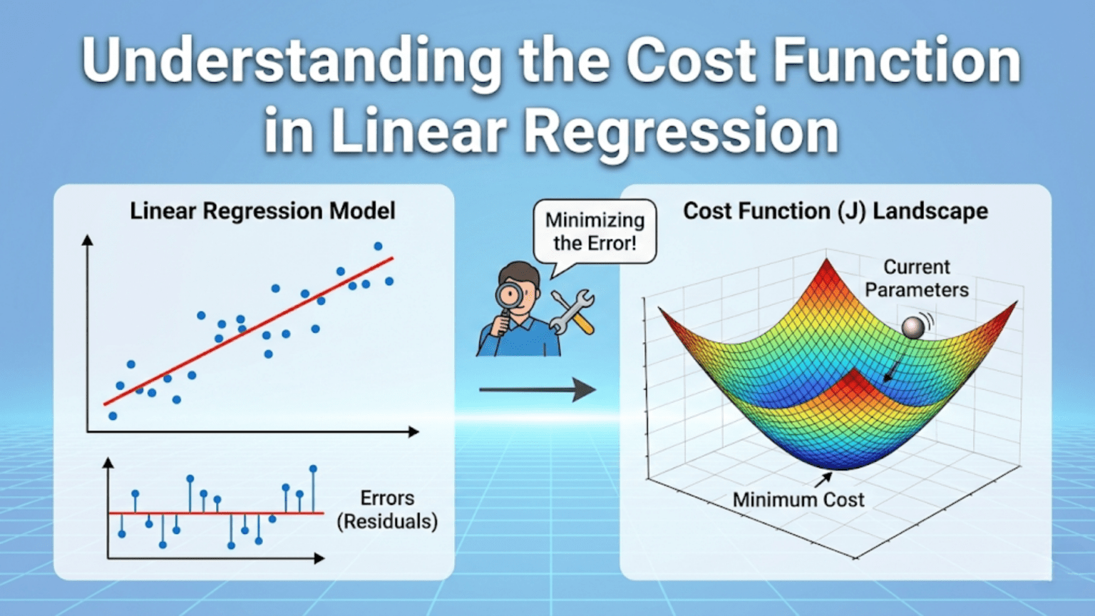
Cost decreased from 55M → 30.15M — model improved!The Loss Landscape: Visualizing the Cost Function
The cost function creates a “landscape” over the parameter space that gradient descent navigates.
One Parameter (w only, b=0)
With one weight parameter, the cost function is a simple parabola:
Cost J(w)
     │         ╲         ╱
     │          ╲       ╱
     │           ╲     ╱
     │            ╲   ╱
     │             ╲ ╱
     │              ✦  ← Global minimum (optimal w)
└───────────────────────── wKey Property: The MSE cost for linear regression is convex — a simple bowl shape with exactly one minimum. Gradient descent will always find it, regardless of starting point.
Two Parameters (w and b)
With both w and b, the cost function is a 3D paraboloid — a bowl in three dimensions:
J(w,b)
    ╱‾‾‾‾‾‾‾‾‾╲
   ╱    ╱‾‾╲    ╲
  │    │ ✦ │    │   ← Minimum at bottom of bowl
   ╲    ╲__╱    ╱
    ╲___________╱

Contour view (top-down):
b │  ╭────╮
  │ ╭──────╮
  │╭────────╮
  │ ╰──────╯   ← Elliptical contours
  │  ╰────╯    ← Center = minimum
└─────────── wContour Lines: Each ring represents a constant cost level. The center (innermost ring) is the optimal (w*, b*) with lowest cost.
What Convexity Means for Training
Convex function properties:
1. Exactly one global minimum (no local minima to get stuck in)
2. Any downhill direction eventually leads to minimum
3. Gradient descent guaranteed to converge

This is why linear regression always finds the optimal solution —
unlike neural networks where the loss landscape is non-convex.How Gradient Descent Navigates the Cost Landscape
The cost function provides the gradient — the direction of steepest ascent — and gradient descent moves in the opposite direction.
The Gradient of MSE
Partial derivative with respect to w:
∂J/∂w = (1/m) × Σᵢ (ŷᵢ − yᵢ) × xᵢ
       = (1/m) × Xᵀ(ŷ − y)      [matrix form]

Interpretation:
If ŷ > y (over-predicting) AND x > 0:
  → Gradient is positive
→ w decreases (correct direction — reduces over-prediction)Partial derivative with respect to b:
∂J/∂b = (1/m) × Σᵢ (ŷᵢ − yᵢ)

Interpretation:
If on average ŷ > y (over-predicting):
  → Gradient is positive
→ b decreases (shifts predictions down)Visual Path Down the Bowl
Cost
 │  Start: high cost
 │  •
 │   ╲
 │    •
 │     ╲
 │      •
 │       ╲
 │        •
 │         ╲__• Converged: low cost
 └────────────────── iterations

Each step: compute gradient → move downhill → cost decreasesComplete Gradient Descent Walk-Through
Simple example: One feature, one training example
x = 2, y = 10
Model: ŷ = wx (b=0 for simplicity)
Learning rate α = 0.1

Initial state: w = 0

Iteration 1:
  Prediction: ŷ = 0 × 2 = 0
  Error: ŷ − y = 0 − 10 = −10
  Cost: J = (1/2)(−10)² = 50

  Gradient: ∂J/∂w = (ŷ−y) × x = −10 × 2 = −20
  Update: w = 0 − 0.1 × (−20) = 2.0

Iteration 2:
  Prediction: ŷ = 2 × 2 = 4
  Error: ŷ − y = 4 − 10 = −6
  Cost: J = (1/2)(−6)² = 18

  Gradient: ∂J/∂w = −6 × 2 = −12
  Update: w = 2.0 − 0.1 × (−12) = 3.2

Iteration 3:
  Prediction: ŷ = 3.2 × 2 = 6.4
  Error: ŷ − y = 6.4 − 10 = −3.6
  Cost: J = (1/2)(−3.6)² = 6.48

  Gradient: ∂J/∂w = −3.6 × 2 = −7.2
  Update: w = 3.2 − 0.1 × (−7.2) = 3.92

... continues converging toward w=5 (true value: y = 5x) ...Cost progression: 50 → 18 → 6.48 → 2.33 → 0.84 → … → ~0
Alternative Cost Functions
MSE is not the only choice. Different problems call for different cost functions.
Mean Absolute Error (MAE)
Formula:
J_MAE = (1/m) × Σᵢ |ŷᵢ − yᵢ|Properties:
- All errors weighted equally regardless of magnitude
- Robust to outliers (large errors don’t dominate)
- Not differentiable at zero (subgradient needed)
- Gradient is constant (±1/m × sign(error))
Comparison with MSE:
Error = 1:    MSE penalty = 1,  MAE penalty = 1  (same)
Error = 10:   MSE penalty = 100, MAE penalty = 10 (MSE 10× harsher)
Error = 100:  MSE penalty = 10000, MAE penalty = 100 (MSE 100× harsher)

MSE penalizes large errors much more aggressively.When to use MAE:
- Data has significant outliers
- Large errors aren’t inherently worse than small ones
- Need median-like behavior (MAE minimizer = conditional median)
When to avoid MAE:
- Gradient descent less stable (non-smooth gradient)
- Usually prefer Huber loss instead
Huber Loss
Formula:
L_δ(ŷ, y) = {
  ½(ŷ−y)²              if |ŷ−y| ≤ δ
  δ(|ŷ−y| − ½δ)        if |ŷ−y| > δ
}The Best of Both Worlds:
Small errors (|error| ≤ δ): behaves like MSE (smooth, penalizes proportionally)
Large errors (|error| > δ): behaves like MAE (linear, doesn't explode)Visual:
Loss
  │     MAE      (linear everywhere)
  │   ╱╱╱
  │  ╱╱╱
  │ ╱╱╱
  │╱──────────── error

  │     MSE      (quadratic everywhere)
  │        ╱╱
  │      ╱╱
  │    ╱╱
  │   ╱╱
  │──╱─────────── error

  │     Huber    (quadratic near 0, linear far out)
  │       ╱╱
  │      ╱╱
  │    ─╱
  │   ╱─
  │──╱──────────── error
└── δ ──┘When to use Huber:
- Regression with outliers (most practical cases)
- When you want outlier-robustness but smooth gradients
- Default choice when MAE seems needed
δ selection: Typically set to a percentile of the expected error magnitude.
Log-Cosh Loss
Formula:
J = (1/m) × Σᵢ log(cosh(ŷᵢ − yᵢ))Properties:
- Approximately ½x² for small errors (like MSE)
- Approximately |x| − log(2) for large errors (like MAE)
- Infinitely differentiable everywhere (even smoother than Huber)
- Less commonly used but useful for XGBoost regression
Quantile Loss (Pinball Loss)
Formula:
L_q(ŷ, y) = {
  q × (y − ŷ)      if y ≥ ŷ
  (1−q) × (ŷ − y)  if y < ŷ
}Purpose: Predict quantiles, not means
Example: With q=0.9, model learns to predict the 90th percentile
Application: Predict upper bound of delivery time
"90% of deliveries will arrive within X hours"When to use: Uncertainty quantification, prediction intervals
Cost Function Comparison Table
| Cost Function | Formula | Outlier Sensitivity | Differentiability | Minimizer | Best For |
|---|---|---|---|---|---|
| MSE | (1/2m)Σ(ŷ−y)² | High | Everywhere | Conditional mean | Clean data, standard regression |
| MAE | (1/m)Σ|ŷ−y| | Low | Except 0 | Conditional median | Outlier-heavy data |
| Huber | Quadratic/linear blend | Medium | Everywhere | Between mean/median | Most practical regression |
| Log-Cosh | (1/m)Σlog(cosh(ŷ−y)) | Low | Everywhere | Near median | Smooth alternative to Huber |
| Quantile | Asymmetric linear | Low | Except 0 | Conditional quantile | Prediction intervals |
Why MSE Creates a Convex Loss Landscape
Understanding convexity is crucial — it’s why linear regression always converges.
Proof of Convexity (Intuitive)
J(w, b) = (1/2m) × Σᵢ (w·xᵢ + b − yᵢ)²

Each term (w·xᵢ + b − yᵢ)² is:
  - A squared linear function of (w, b)
  - Therefore convex in (w, b)

Sum of convex functions = convex

Therefore J is convex — guaranteed single minimum.What Convexity Guarantees
Convex cost function guarantees:
✓ Only one global minimum (no local minima)
✓ Gradient descent will find it
✓ Any learning rate (small enough) eventually converges
✓ Stopping at any local minimum = stopping at global minimum

Non-convex (neural networks):
✗ Many local minima
✗ Gradient descent may get stuck
✗ Different initializations give different results
✗ Training is much harderPractical Python: Exploring the Cost Function
import numpy as np
import matplotlib.pyplot as plt

# ── Dataset ──────────────────────────────────────────────────
np.random.seed(42)
m = 50
X = np.linspace(0, 10, m)
y = 2.5 * X + 5 + np.random.normal(0, 3, m)  # true: w=2.5, b=5


# ── Cost functions ────────────────────────────────────────────
def mse_cost(X, y, w, b):
    y_pred = w * X + b
    return (1 / (2 * len(y))) * np.sum((y_pred - y) ** 2)

def mae_cost(X, y, w, b):
    y_pred = w * X + b
    return np.mean(np.abs(y_pred - y))

def huber_cost(X, y, w, b, delta=5.0):
    errors = w * X + b - y
    is_small = np.abs(errors) <= delta
    sq = 0.5 * errors ** 2
    lin = delta * (np.abs(errors) - 0.5 * delta)
    return np.mean(np.where(is_small, sq, lin))


# ── 1. Visualise cost as function of w (fix b at true value) ─
w_range = np.linspace(-2, 7, 200)
b_fixed = 5.0

costs_mse  = [mse_cost(X, y, w, b_fixed)  for w in w_range]
costs_mae  = [mae_cost(X, y, w, b_fixed)   for w in w_range]
costs_hub  = [huber_cost(X, y, w, b_fixed) for w in w_range]

fig, axes = plt.subplots(1, 3, figsize=(15, 4))

for ax, costs, name, color in zip(
        axes,
        [costs_mse, costs_mae, costs_hub],
        ['MSE Cost', 'MAE Cost', 'Huber Cost'],
        ['steelblue', 'coral', 'seagreen']):
    ax.plot(w_range, costs, color=color, linewidth=2)
    ax.axvline(x=2.5, color='gray', linestyle='--', alpha=0.7,
               label='True w=2.5')
    ax.set_xlabel('Weight w')
    ax.set_ylabel('Cost')
    ax.set_title(name)
    ax.legend()
    ax.grid(True, alpha=0.3)

plt.tight_layout()
plt.show()


# ── 2. 3D cost surface over (w, b) space ─────────────────────
w_grid = np.linspace(0, 5, 80)
b_grid = np.linspace(-5, 15, 80)
W, B   = np.meshgrid(w_grid, b_grid)

# Vectorised computation
J_grid = np.zeros_like(W)
for i in range(W.shape[0]):
    for j in range(W.shape[1]):
        J_grid[i, j] = mse_cost(X, y, W[i, j], B[i, j])

fig = plt.figure(figsize=(14, 5))

# 3D surface
ax1 = fig.add_subplot(121, projection='3d')
ax1.plot_surface(W, B, J_grid, cmap='viridis', alpha=0.85)
ax1.set_xlabel('w (weight)')
ax1.set_ylabel('b (bias)')
ax1.set_zlabel('Cost J(w,b)')
ax1.set_title('MSE Cost Surface')

# Contour plot
ax2 = fig.add_subplot(122)
contour = ax2.contourf(W, B, J_grid, levels=30, cmap='viridis')
plt.colorbar(contour, ax=ax2)
ax2.scatter([2.5], [5], color='red', s=100, zorder=5,
            label='True optimum')
ax2.set_xlabel('w (weight)')
ax2.set_ylabel('b (bias)')
ax2.set_title('MSE Cost Contours')
ax2.legend()

plt.tight_layout()
plt.show()


# ── 3. Trace gradient descent path on contour plot ───────────
def gradient_descent_trace(X, y, w_init, b_init,
                            lr=0.01, n_iter=100):
    """Run GD and record (w, b, cost) at each step."""
    w, b    = w_init, b_init
    history = [(w, b, mse_cost(X, y, w, b))]

    for _ in range(n_iter):
        y_pred = w * X + b
        errors = y_pred - y
        dw = (1 / len(y)) * np.sum(errors * X)
        db = (1 / len(y)) * np.sum(errors)
        w -= lr * dw
        b -= lr * db
        history.append((w, b, mse_cost(X, y, w, b)))

    return np.array(history)

trace = gradient_descent_trace(X, y,
                                w_init=0.0, b_init=0.0,
                                lr=0.005, n_iter=300)

fig, axes = plt.subplots(1, 2, figsize=(14, 5))

# Contour + path
ax = axes[0]
contour = ax.contourf(W, B, J_grid, levels=30, cmap='Blues')
plt.colorbar(contour, ax=ax)
ax.plot(trace[:, 0], trace[:, 1],
        'r.-', markersize=4, linewidth=1, label='GD path')
ax.scatter(trace[0, 0],  trace[0, 1],  color='green',
           s=100, zorder=6, label='Start')
ax.scatter(trace[-1, 0], trace[-1, 1], color='red',
           s=100, zorder=6, label='End')
ax.scatter([2.5], [5], color='gold', s=150, marker='*',
           zorder=7, label='True optimum')
ax.set_xlabel('w')
ax.set_ylabel('b')
ax.set_title('Gradient Descent Path on Cost Contours')
ax.legend(fontsize=8)

# Cost over iterations
ax = axes[1]
ax.plot(trace[:, 2], color='steelblue', linewidth=2)
ax.set_xlabel('Iteration')
ax.set_ylabel('Cost J(w,b)')
ax.set_title('Cost Decreasing During Training')
ax.grid(True, alpha=0.3)

plt.tight_layout()
plt.show()

print(f"Learned w = {trace[-1, 0]:.4f}  (true = 2.5)")
print(f"Learned b = {trace[-1, 1]:.4f}  (true = 5.0)")
print(f"Final cost: {trace[-1, 2]:.4f}")Effect of Outliers on Different Cost Functions
# Create dataset with one severe outlier
np.random.seed(1)
X_out = np.array([1, 2, 3, 4, 5, 6, 7, 8, 9, 10], dtype=float)
y_out = np.array([2, 4, 6, 8, 10, 12, 14, 16, 18, 100])  # Last is outlier

# Fit with MSE (from scratch)
def fit_gd(X, y, cost_fn, lr=0.001, n_iter=5000):
    w, b = 0.0, 0.0
    for _ in range(n_iter):
        y_pred = w * X + b
        errors = y_pred - y
        if cost_fn == 'mse':
            dw = (1/len(y)) * np.sum(errors * X)
            db = (1/len(y)) * np.sum(errors)
        else:  # mae
            signs = np.sign(errors)
            dw = (1/len(y)) * np.sum(signs * X)
            db = (1/len(y)) * np.sum(signs)
        w -= lr * dw
        b -= lr * db
    return w, b

w_mse, b_mse = fit_gd(X_out, y_out, 'mse', lr=0.0001, n_iter=20000)
w_mae, b_mae = fit_gd(X_out, y_out, 'mae', lr=0.001,  n_iter=20000)

print("Effect of outlier on different cost functions:")
print(f"  MSE fit:  w={w_mse:.3f}, b={b_mse:.3f}  (pulled toward outlier)")
print(f"  MAE fit:  w={w_mae:.3f}, b={b_mae:.3f}  (more robust)")
print(f"  True:     w=2.000, b=0.000")

# Visualise
x_plot = np.linspace(0, 11, 100)
plt.figure(figsize=(8, 5))
plt.scatter(X_out[:-1], y_out[:-1], color='steelblue',
            s=60, label='Normal points', zorder=5)
plt.scatter(X_out[-1:], y_out[-1:], color='red',
            s=120, marker='*', label='Outlier', zorder=6)
plt.plot(x_plot, w_mse * x_plot + b_mse,
         'orange', linewidth=2, label=f'MSE fit (w={w_mse:.2f})')
plt.plot(x_plot, w_mae * x_plot + b_mae,
         'green',  linewidth=2, label=f'MAE fit (w={w_mae:.2f})')
plt.plot(x_plot, 2 * x_plot,
         'gray', linewidth=1.5, linestyle='--', label='True line (w=2.0)')
plt.xlabel('x')
plt.ylabel('y')
plt.title('MSE vs MAE: Sensitivity to Outliers')
plt.legend()
plt.grid(True, alpha=0.3)
plt.tight_layout()
plt.show()What this demonstrates: MSE is pulled significantly toward the outlier because it squares the error — a residual of 80 contributes 6,400 to the cost, dominating the optimization. MAE penalizes that same error linearly (80), giving it no more relative influence than a cluster of smaller errors.
The Gradient Interpretation: What Each Formula Means
The gradient formulas have intuitive meaning worth understanding deeply.
Weight Gradient
∂J/∂w = (1/m) × Σᵢ (ŷᵢ − yᵢ) × xᵢReading this formula:
(ŷᵢ − yᵢ): Signed error for example i (positive = over-predicted, negative = under-predicted)× xᵢ: Weight the error by the feature valueΣᵢ / m: Average over all examples
Intuition:
- If the model over-predicts (ŷ > y) on examples with large x: gradient is positive → decrease w
- If the model under-predicts (ŷ < y) on examples with large x: gradient is negative → increase w
- Feature values x act as amplifiers: large x → that example contributes more to weight adjustment
Bias Gradient
∂J/∂b = (1/m) × Σᵢ (ŷᵢ − yᵢ)Reading this formula:
- Simply the average signed error across all examples
- If average error is positive (consistently over-predicting): decrease b
- If average error is negative (consistently under-predicting): increase b
- The bias is a vertical shift — it corrects systematic over or under-prediction
Common Mistakes and How to Avoid Them
Mistake 1: Not Checking the Cost is Decreasing
Always plot the cost curve. If cost increases or oscillates, something is wrong.
# Check after every training run
if model.cost_history[-1] > model.cost_history[0]:
print("Warning: cost increased! Check learning rate and data.")Mistake 2: Forgetting to Divide by m
# Wrong (cost grows with dataset size)
cost = np.sum((y_pred - y) ** 2)

# Right (scale-independent)
cost = np.mean((y_pred - y) ** 2)
# or equivalently:
cost = (1/m) * np.sum((y_pred - y) ** 2)Mistake 3: Using Raw MSE Units to Compare Models
MSE is in squared units (dollars², degrees²). Use RMSE for interpretable comparison:
rmse = np.sqrt(mean_squared_error(y_test, y_pred))
print(f"Average error: ${rmse:,.0f}") # InterpretableMistake 4: Ignoring Outliers
If your data has outliers, MSE will fit them at the expense of regular points. Either:
- Clean the outliers
- Use Huber loss or MAE instead
Mistake 5: Comparing Costs Across Different Datasets
Cost values are not comparable across datasets with different scales or sizes. Always use R² or normalised metrics for comparison.
Conclusion: The Compass of Machine Learning
The cost function is not just a formula — it is the definition of what your model is trying to achieve. Every element of the cost function is a design decision: what errors to penalize, how much to penalize large errors versus small ones, whether outliers should be influential, and whether you want to predict means or quantiles.
Understanding MSE deeply means understanding:
Why it works: Squaring errors eliminates sign issues, creates smooth gradients, and creates a convex landscape that gradient descent can navigate reliably to the global minimum.
What it optimizes: MSE minimization finds the conditional mean — the model predicts the average y given x. This is the right objective for most regression problems.
When to replace it: Heavy outliers in your data? Use Huber. Need prediction intervals? Use quantile loss. Want median predictions? Use MAE.
How it connects forward: The cost function in a neural network is the same concept applied to deeper architectures. Cross-entropy for classification, MSE for regression, custom losses for specialized tasks — all are cost functions guiding gradient descent toward better predictions.
The cost function is the bridge between data and learning. It translates raw prediction errors into the gradient signal that drives every weight update in every machine learning model ever trained. Master it here in the simplest context of linear regression, and you’ve mastered the central concept that makes machine learning work.